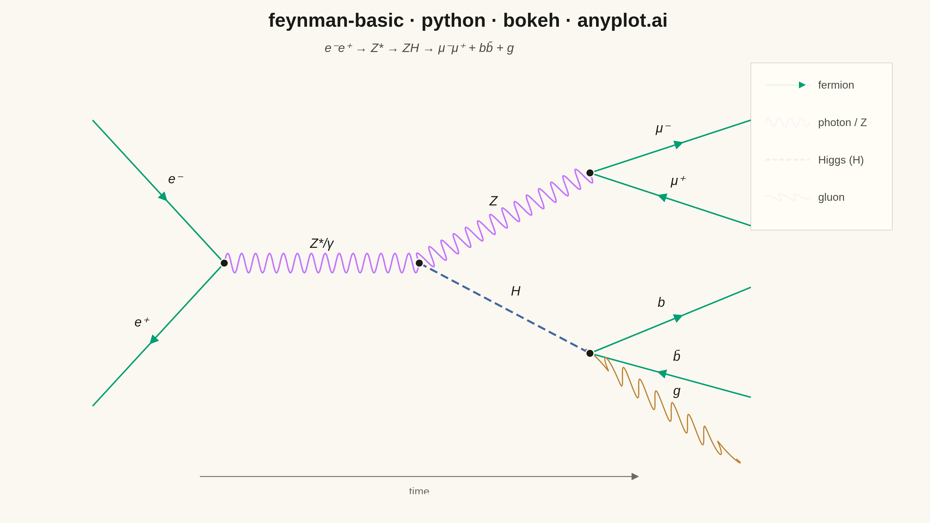
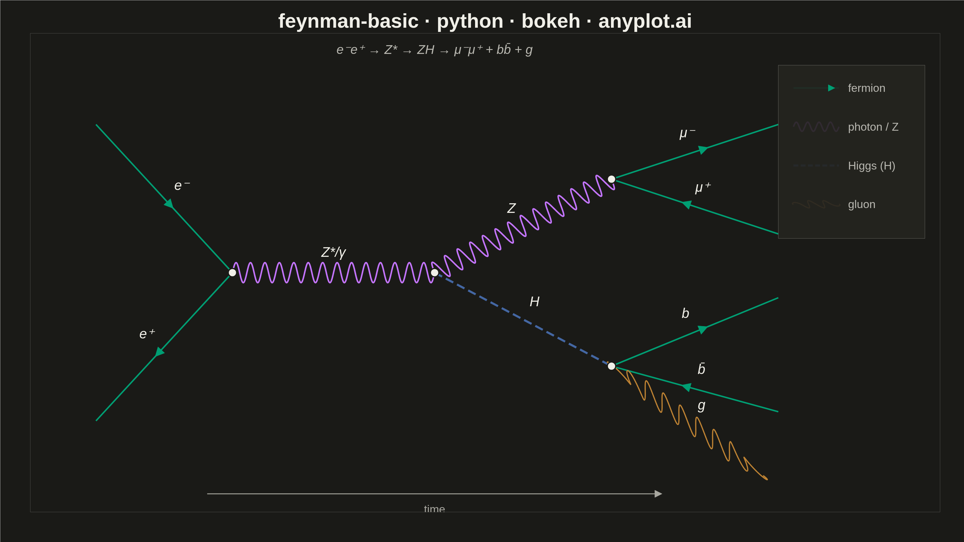
A Feynman diagram visualizes interactions between subatomic particles in quantum field theory. Different line styles represent different particle types: straight lines for fermions (electrons, quarks), wavy lines for photons, curly/looped lines for gluons, and dashed lines for scalar bosons (e.g., Higgs). Lines meet at vertices representing interaction points. Invented by Richard Feynman, these diagrams are both a computational tool and a cultural icon of modern physics.
""" anyplot.ai
feynman-basic: Feynman Diagram for Particle Interactions
Library: bokeh 3.9.0 | Python 3.13.13
Quality: 93/100 | Updated: 2026-06-03
"""

import os
import time
from pathlib import Path

import numpy as np
from bokeh.io import output_file, save
from bokeh.models import Arrow, BoxAnnotation, Label, NormalHead, Range1d
from bokeh.plotting import figure
from selenium import webdriver
from selenium.webdriver.chrome.options import Options


# Theme-adaptive chrome tokens
THEME = os.getenv("ANYPLOT_THEME", "light")
PAGE_BG = "#FAF8F1" if THEME == "light" else "#1A1A17"
ELEVATED_BG = "#FFFDF6" if THEME == "light" else "#242420"
INK = "#1A1A17" if THEME == "light" else "#F0EFE8"
INK_SOFT = "#4A4A44" if THEME == "light" else "#B8B7B0"
INK_MUTED = "#6B6A63" if THEME == "light" else "#A8A79F"

# Imprint palette — canonical order, positions 1-4
FERMION_COLOR = "#009E73"  # pos 1: brand green  — fermion lines (e, μ, b quarks)
PHOTON_COLOR = "#C475FD"  # pos 2: lavender     — wavy photon/Z propagators
BOSON_COLOR = "#4467A3"  # pos 3: blue         — dashed scalar Higgs
GLUON_COLOR = "#BD8233"  # pos 4: ochre        — curly gluon radiation

TYPE_COLORS = {"fermion": FERMION_COLOR, "photon": PHOTON_COLOR, "boson": BOSON_COLOR, "gluon": GLUON_COLOR}

# Data — Higgs-strahlung: e⁻e⁺ → Z* → ZH → μ⁻μ⁺ + bb̄ + g
# Coordinates spread wide to fill the 16:9 canvas (x: 0.3–13.8, y: −0.7–7.0)
v1 = (3.0, 3.75)  # e⁻e⁺ annihilation vertex
v2 = (7.0, 3.75)  # virtual Z*/γ endpoint + ZH-splitting vertex
v3 = (10.5, 5.8)  # Z → μ⁻μ⁺ decay vertex
v4 = (10.5, 1.7)  # H → bb̄g decay vertex

propagators = [
    # Incoming fermions
    {"start": (0.3, 7.0), "end": v1, "type": "fermion", "label": "e⁻", "arrow": "forward"},
    {"start": (0.3, 0.5), "end": v1, "type": "fermion", "label": "e⁺", "arrow": "backward"},
    # Virtual and real vector bosons (wavy)
    {"start": v1, "end": v2, "type": "photon", "label": "Z*/γ"},
    {"start": v2, "end": v3, "type": "photon", "label": "Z"},
    # Scalar Higgs (dashed)
    {"start": v2, "end": v4, "type": "boson", "label": "H"},
    # Z decay products
    {"start": v3, "end": (13.8, 7.0), "type": "fermion", "label": "μ⁻", "arrow": "forward"},
    {"start": v3, "end": (13.8, 4.6), "type": "fermion", "label": "μ⁺", "arrow": "backward"},
    # H decay products
    {"start": v4, "end": (13.8, 3.2), "type": "fermion", "label": "b", "arrow": "forward"},
    {"start": v4, "end": (13.8, 0.7), "type": "fermion", "label": "b̄", "arrow": "backward"},
    {"start": v4, "end": (13.5, -0.7), "type": "gluon", "label": "g"},
]

# Canvas — 3200×1800 (landscape), title 43 chars < 67 baseline so no size scaling
title_str = "feynman-basic · python · bokeh · anyplot.ai"

p = figure(
    width=3200,
    height=1800,
    title=title_str,
    x_range=Range1d(-1.0, 17.0),
    y_range=Range1d(-1.5, 9.0),
    toolbar_location=None,
    min_border_top=110,
    min_border_bottom=100,
    min_border_left=100,
    min_border_right=80,
)

p.axis.visible = False
p.grid.visible = False
p.outline_line_color = None

p.background_fill_color = PAGE_BG
p.border_fill_color = PAGE_BG
p.title.text_font_size = "50pt"
p.title.text_color = INK
p.title.align = "center"

# Draw propagators
for prop in propagators:
    x0, y0 = prop["start"]
    x1, y1 = prop["end"]
    dx, dy = x1 - x0, y1 - y0
    length = np.sqrt(dx**2 + dy**2)
    color = TYPE_COLORS[prop["type"]]
    perp_x, perp_y = -dy / length, dx / length

    if prop["type"] == "fermion":
        p.line([x0, x1], [y0, y1], line_width=5, color=color)
        # Directional arrow at midpoint (forward = particle, backward = antiparticle)
        mid_x, mid_y = (x0 + x1) / 2, (y0 + y1) / 2
        off = 0.28
        if prop.get("arrow") == "backward":
            sx, sy = mid_x + off * dx / length, mid_y + off * dy / length
            ex, ey = mid_x - off * dx / length, mid_y - off * dy / length
        else:
            sx, sy = mid_x - off * dx / length, mid_y - off * dy / length
            ex, ey = mid_x + off * dx / length, mid_y + off * dy / length
        p.add_layout(
            Arrow(
                end=NormalHead(size=30, fill_color=color, line_color=color),
                x_start=sx,
                y_start=sy,
                x_end=ex,
                y_end=ey,
                line_width=0,
                line_alpha=0,
            )
        )

    elif prop["type"] == "photon":
        n_waves = max(6, int(length * 3.5))
        t = np.linspace(0, 1, 600)
        wave = 0.22 * np.sin(2 * np.pi * n_waves * t)
        p.line(
            (x0 + t * dx + wave * perp_x).tolist(), (y0 + t * dy + wave * perp_y).tolist(), line_width=5, color=color
        )

    elif prop["type"] == "gluon":
        n_coils = max(5, int(length * 2.5))
        t = np.linspace(0, 1, 1400)
        angle = 2 * np.pi * n_coils * t
        taper = np.minimum(t * 5, 1.0) * np.minimum((1 - t) * 5, 1.0)
        eff_t = t - (0.18 * 1.2 / length) * np.sin(angle)
        p.line(
            (x0 + eff_t * dx + 0.18 * np.sin(angle) * perp_x * taper).tolist(),
            (y0 + eff_t * dy + 0.18 * np.sin(angle) * perp_y * taper).tolist(),
            line_width=4,
            color=color,
        )

    elif prop["type"] == "boson":
        p.line([x0, x1], [y0, y1], line_width=7, color=color, line_dash=[28, 14])

    # Particle label — offset perpendicular to the propagator
    mid_x, mid_y = (x0 + x1) / 2, (y0 + y1) / 2
    p.add_layout(
        Label(
            x=mid_x + 0.45 * perp_x,
            y=mid_y + 0.45 * perp_y,
            text=prop["label"],
            text_font_size="34pt",
            text_font_style="italic",
            text_color=INK,
            text_align="center",
            text_baseline="middle",
        )
    )

# Vertex dots (white-bordered filled circles)
verts_x = [v1[0], v2[0], v3[0], v4[0]]
verts_y = [v1[1], v2[1], v3[1], v4[1]]
p.scatter(verts_x, verts_y, size=28, color=INK, line_color=PAGE_BG, line_width=4)

# Legend — upper-right corner, past the outgoing particle endpoints
p.add_layout(
    BoxAnnotation(
        left=13.8,
        right=16.7,
        bottom=4.5,
        top=8.3,
        fill_color=ELEVATED_BG,
        fill_alpha=0.92,
        line_color=INK_SOFT,
        line_width=1,
        line_alpha=0.5,
    )
)

legend_entries = [
    ("fermion", FERMION_COLOR, "solid"),
    ("photon / Z", PHOTON_COLOR, "wavy"),
    ("Higgs (H)", BOSON_COLOR, "dashed"),
    ("gluon", GLUON_COLOR, "curly"),
]
leg_x0, leg_len = 14.1, 0.9
for i, (name, color, style) in enumerate(legend_entries):
    y = 7.8 - i * 0.85
    lx1 = leg_x0 + leg_len

    if style == "solid":
        p.line([leg_x0, lx1], [y, y], line_width=5, color=color)
        p.add_layout(
            Arrow(
                end=NormalHead(size=22, fill_color=color, line_color=color),
                x_start=leg_x0 + 0.22,
                y_start=y,
                x_end=lx1 - 0.08,
                y_end=y,
                line_width=0,
                line_alpha=0,
            )
        )
    elif style == "wavy":
        t_l = np.linspace(0, 1, 200)
        p.line(
            (leg_x0 + t_l * leg_len).tolist(),
            (y + 0.10 * np.sin(2 * np.pi * 4 * t_l)).tolist(),
            line_width=5,
            color=color,
        )
    elif style == "curly":
        t_l = np.linspace(0, 1, 400)
        al = 2 * np.pi * 3 * t_l
        tap = np.minimum(t_l * 5, 1.0) * np.minimum((1 - t_l) * 5, 1.0)
        eff = t_l - (0.08 / leg_len) * np.sin(al)
        p.line((leg_x0 + eff * leg_len).tolist(), (y + 0.08 * np.sin(al) * tap).tolist(), line_width=4, color=color)
    elif style == "dashed":
        p.line([leg_x0, lx1], [y, y], line_width=7, color=color, line_dash=[16, 8])

    p.add_layout(
        Label(
            x=lx1 + 0.18,
            y=y,
            text=name,
            text_font_size="28pt",
            text_color=INK_SOFT,
            text_align="left",
            text_baseline="middle",
        )
    )

# Time axis arrow along the bottom
p.add_layout(
    Arrow(
        end=NormalHead(size=24, fill_color=INK_MUTED, line_color=INK_MUTED),
        x_start=2.5,
        y_start=-1.1,
        x_end=11.5,
        y_end=-1.1,
        line_width=3,
        line_color=INK_MUTED,
    )
)
p.add_layout(
    Label(
        x=7.0,
        y=-1.3,
        text="time",
        text_font_size="28pt",
        text_color=INK_MUTED,
        text_align="center",
        text_baseline="top",
    )
)

# Process equation at top center
p.add_layout(
    Label(
        x=7.0,
        y=8.65,
        text="e⁻e⁺ → Z* → ZH → μ⁻μ⁺ + bb̄ + g",
        text_font_size="32pt",
        text_color=INK_SOFT,
        text_font_style="italic",
        text_align="center",
        text_baseline="middle",
    )
)

# Save HTML (interactive catalog artifact)
output_file(f"plot-{THEME}.html")
save(p)

# Inject CSS reset so the figure starts at y=0 with no body margins
html_path = Path(f"plot-{THEME}.html")
html_src = html_path.read_text()
css_reset = "<style>html,body{margin:0;padding:0;overflow:hidden}</style>"
html_path.write_text(html_src.replace("<head>", f"<head>{css_reset}"))

# Screenshot with headless Chrome — set outer window to 3200×1939 so that
# the inner viewport (after Chrome's 139px internal overhead) is exactly 3200×1800.
W, H = 3200, 1800
OUTER_H = 1939  # W × (H + 139px Chrome overhead) = correct inner viewport of H
opts = Options()
for arg in (
    "--headless=new",
    "--no-sandbox",
    "--disable-dev-shm-usage",
    "--disable-gpu",
    f"--window-size={W},{OUTER_H}",
    "--hide-scrollbars",
):
    opts.add_argument(arg)
driver = webdriver.Chrome(options=opts)
driver.set_window_size(W, OUTER_H)
driver.get(f"file://{html_path.resolve()}")
time.sleep(3)
driver.save_screenshot(f"plot-{THEME}.png")
driver.quit()
Runnable source as JSON, for any HTTP client: https://api.anyplot.ai/specs/feynman-basic/bokeh/code. Any spec id and library id listed in llms-full.txt fit the same URL shape; every URL below is complete and callable.
{
  "spec_id": "feynman-basic",
  "language": "python",
  "library": "bokeh",
  "page": "https://anyplot.ai/feynman-basic/python/bokeh",
  "hub": "https://anyplot.ai/feynman-basic",
  "code_json": "https://api.anyplot.ai/specs/feynman-basic/bokeh/code",
  "spec_json": "https://api.anyplot.ai/specs/feynman-basic",
  "render_light_png": "https://storage.googleapis.com/anyplot-images/plots/feynman-basic/python/bokeh/plot-light.png",
  "render_dark_png": "https://storage.googleapis.com/anyplot-images/plots/feynman-basic/python/bokeh/plot-dark.png",
  "interactive_light_html": "https://storage.googleapis.com/anyplot-images/plots/feynman-basic/python/bokeh/plot-light.html",
  "interactive_dark_html": "https://storage.googleapis.com/anyplot-images/plots/feynman-basic/python/bokeh/plot-dark.html",
  "quality_score": 93.0,
  "license": "MIT",
  "guide": "https://anyplot.ai/llms.txt"
}
Part of Feynman Diagram for Particle Interactions on anyplot.ai.