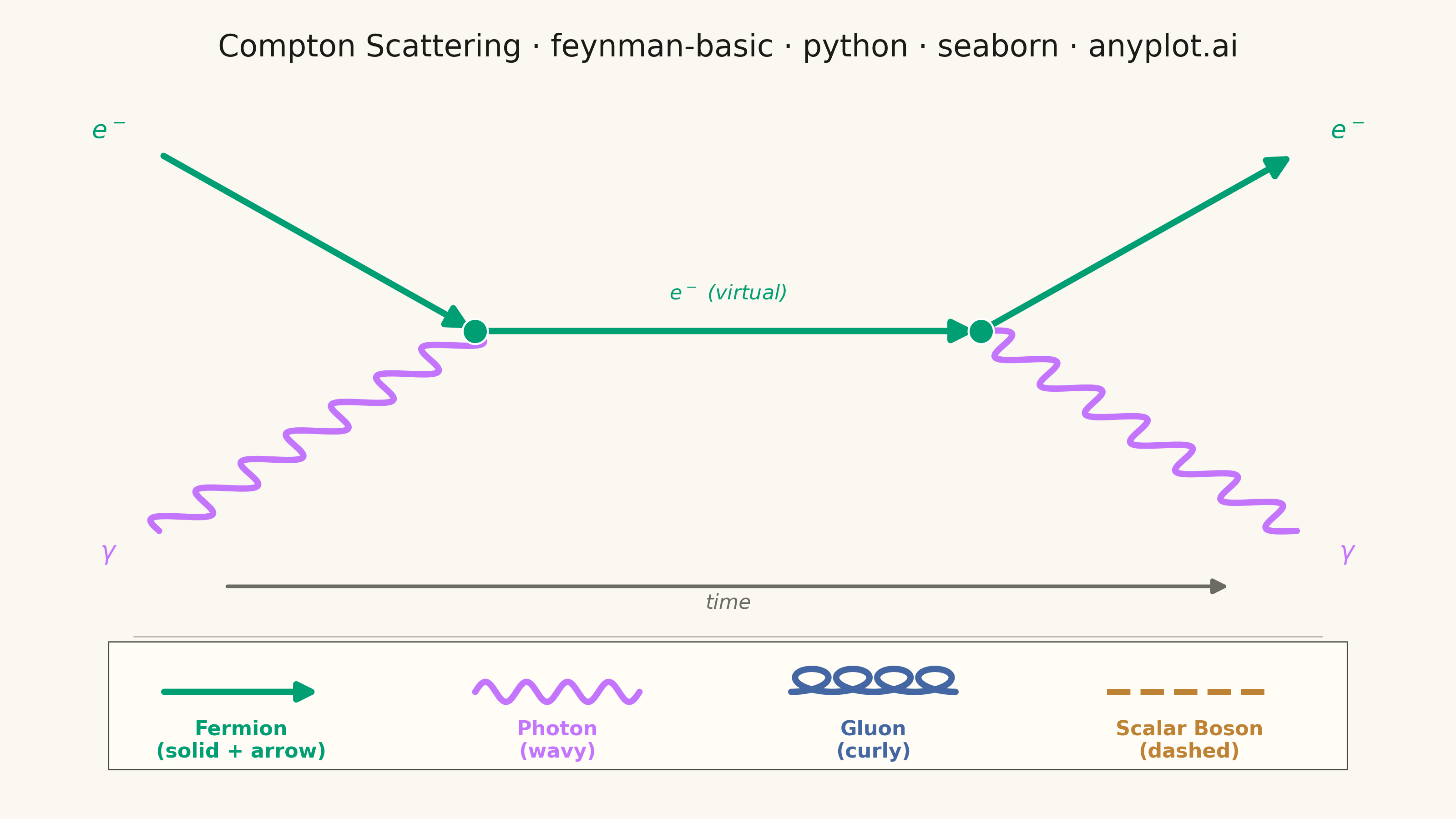
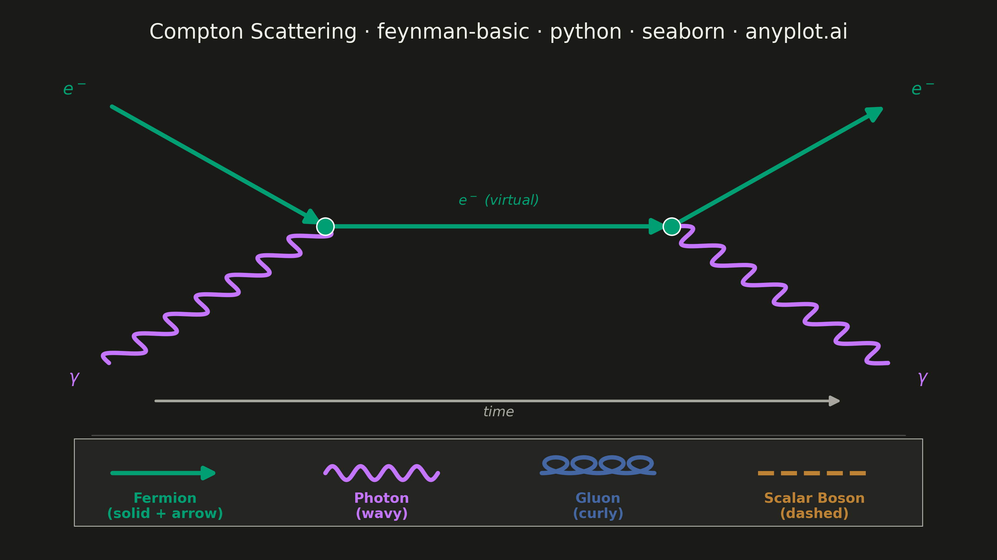
A Feynman diagram visualizes interactions between subatomic particles in quantum field theory. Different line styles represent different particle types: straight lines for fermions (electrons, quarks), wavy lines for photons, curly/looped lines for gluons, and dashed lines for scalar bosons (e.g., Higgs). Lines meet at vertices representing interaction points. Invented by Richard Feynman, these diagrams are both a computational tool and a cultural icon of modern physics.
""" anyplot.ai
feynman-basic: Feynman Diagram for Particle Interactions
Library: seaborn 0.13.2 | Python 3.13.13
Quality: 89/100 | Updated: 2026-06-03
"""

import os
import sys


# Remove this directory from sys.path to prevent local matplotlib.py from
# shadowing the installed package (implementations dir contains other lib files)
_here = os.path.realpath(os.path.dirname(os.path.abspath(__file__)))
sys.path = [p for p in sys.path if os.path.realpath(p if p else os.getcwd()) != _here]

import matplotlib.patches as mpatches
import matplotlib.pyplot as plt
import numpy as np
import pandas as pd
import seaborn as sns


# Theme tokens
THEME = os.getenv("ANYPLOT_THEME", "light")
PAGE_BG = "#FAF8F1" if THEME == "light" else "#1A1A17"
ELEVATED_BG = "#FFFDF6" if THEME == "light" else "#242420"
INK = "#1A1A17" if THEME == "light" else "#F0EFE8"
INK_SOFT = "#4A4A44" if THEME == "light" else "#B8B7B0"
INK_MUTED = "#6B6A63" if THEME == "light" else "#A8A79F"

# Imprint palette — canonical order, first series always #009E73
FERMION = "#009E73"  # Imprint position 1 (brand green) — electrons
PHOTON = "#C475FD"  # Imprint position 2 (lavender)    — photons
GLUON = "#4467A3"  # Imprint position 3 (blue)         — gluons (reference only)
SCALAR = "#BD8233"  # Imprint position 4 (ochre)        — scalar bosons (reference only)

IMPRINT_PALETTE = [FERMION, PHOTON, GLUON, SCALAR, "#AE3030", "#2ABCCD", "#954477", "#99B314"]
sns.set_theme(style="white", rc={"figure.facecolor": PAGE_BG, "axes.facecolor": PAGE_BG, "text.color": INK})
sns.set_palette(IMPRINT_PALETTE)

# Canvas — landscape 3200 × 1800 px
fig, ax = plt.subplots(figsize=(8, 4.5), dpi=400, facecolor=PAGE_BG)
ax.set_facecolor(PAGE_BG)

# === Main Diagram: Compton Scattering (e⁻ + γ → e⁻ + γ) ===
# t-channel: incoming electron absorbs the photon (v1), propagates as a virtual
# electron, then emits the scattered photon at v2
v1 = np.array([0.30, 0.58])  # absorption vertex
v2 = np.array([0.70, 0.58])  # emission vertex

e_in = np.array([0.05, 0.90])  # incoming electron endpoint
e_out = np.array([0.95, 0.90])  # outgoing electron endpoint
g_in = np.array([0.05, 0.22])  # incoming photon endpoint
g_out = np.array([0.95, 0.22])  # outgoing photon endpoint

arrow_kw = {"arrowstyle": "-|>", "color": FERMION, "lw": 2.5, "mutation_scale": 18}

# Fermion lines with directional arrows
ax.annotate("", xy=v1, xytext=e_in, arrowprops=arrow_kw)  # e⁻(in) → v1
ax.annotate("", xy=v2, xytext=v1, arrowprops=arrow_kw)  # v1 → v2 (virtual e⁻)
ax.annotate("", xy=e_out, xytext=v2, arrowprops=arrow_kw)  # v2 → e⁻(out)

# Incoming photon wavy line
t = np.linspace(0, 1, 400)
d_gin = v1 - g_in
perp_gin = np.array([-d_gin[1], d_gin[0]]) / np.linalg.norm(d_gin)
wave_gin = 0.018 * np.sin(2 * np.pi * 7 * t)
gamma_in_df = pd.DataFrame(
    {"x": g_in[0] + t * d_gin[0] + wave_gin * perp_gin[0], "y": g_in[1] + t * d_gin[1] + wave_gin * perp_gin[1]}
)
sns.lineplot(data=gamma_in_df, x="x", y="y", ax=ax, color=PHOTON, linewidth=2.5, sort=False, legend=False)

# Outgoing photon wavy line
d_gout = g_out - v2
perp_gout = np.array([-d_gout[1], d_gout[0]]) / np.linalg.norm(d_gout)
wave_gout = 0.018 * np.sin(2 * np.pi * 7 * t)
gamma_out_df = pd.DataFrame(
    {"x": v2[0] + t * d_gout[0] + wave_gout * perp_gout[0], "y": v2[1] + t * d_gout[1] + wave_gout * perp_gout[1]}
)
sns.lineplot(data=gamma_out_df, x="x", y="y", ax=ax, color=PHOTON, linewidth=2.5, sort=False, legend=False)

# Interaction vertex dots
vertex_df = pd.DataFrame({"x": [v1[0], v2[0]], "y": [v1[1], v2[1]]})
sns.scatterplot(data=vertex_df, x="x", y="y", ax=ax, color=FERMION, s=100, zorder=5, legend=False)

# Particle labels
lkw_e = {"fontsize": 10, "fontweight": "bold", "ha": "center", "va": "center", "color": FERMION}
lkw_g = {"fontsize": 10, "fontweight": "bold", "ha": "center", "va": "center", "color": PHOTON}
ax.text(e_in[0] - 0.04, e_in[1] + 0.04, r"$e^-$", **lkw_e)
ax.text(e_out[0] + 0.04, e_out[1] + 0.04, r"$e^-$", **lkw_e)
ax.text(g_in[0] - 0.04, g_in[1] - 0.04, r"$\gamma$", **lkw_g)
ax.text(g_out[0] + 0.04, g_out[1] - 0.04, r"$\gamma$", **lkw_g)
ax.text(0.50, 0.63, r"$e^-$ (virtual)", fontsize=8, color=FERMION, ha="center", va="bottom", style="italic")

# Time arrow
ax.annotate(
    "",
    xy=(0.90, 0.12),
    xytext=(0.10, 0.12),
    arrowprops={"arrowstyle": "-|>", "color": INK_MUTED, "lw": 1.5, "mutation_scale": 12},
)
ax.text(0.50, 0.08, "time", fontsize=8, color=INK_MUTED, ha="center", style="italic")

# Separator between main diagram and reference legend
ax.plot([0.03, 0.97], [0.03, 0.03], color=INK_SOFT, lw=0.5, alpha=0.4)

# Elevated card background for reference legend (visual separation)
legend_card = mpatches.FancyBboxPatch(
    (0.01, -0.21),
    0.98,
    0.23,
    boxstyle="round,pad=0.0",
    facecolor=ELEVATED_BG,
    edgecolor=INK_SOFT,
    linewidth=0.5,
    alpha=1.0,
    transform=ax.transData,
    zorder=0.5,
)
ax.add_patch(legend_card)

# === Reference legend: all 4 particle line styles ===
ref_y = -0.07
ref_spans = [(0.05, 0.18), (0.30, 0.43), (0.55, 0.68), (0.80, 0.93)]
ref_names = ["Fermion\n(solid + arrow)", "Photon\n(wavy)", "Gluon\n(curly)", "Scalar Boson\n(dashed)"]
ref_cols = [FERMION, PHOTON, GLUON, SCALAR]

# Fermion reference
ax.annotate(
    "",
    xy=(ref_spans[0][1], ref_y),
    xytext=(ref_spans[0][0], ref_y),
    arrowprops={"arrowstyle": "-|>", "color": FERMION, "lw": 2.5, "mutation_scale": 15},
)

# Photon reference — wavy
tr = np.linspace(0, 1, 300)
xs0, xs1 = ref_spans[1]
photon_ref = pd.DataFrame({"x": xs0 + tr * (xs1 - xs0), "y": ref_y + 0.018 * np.sin(2 * np.pi * 4 * tr)})
sns.lineplot(data=photon_ref, x="x", y="y", ax=ax, color=PHOTON, linewidth=2.5, sort=False, legend=False)

# Gluon reference — curly (cycloid parameterization)
tg = np.linspace(0, 1, 1000)
xs0, xs1 = ref_spans[2]
span_g = xs1 - xs0
n_coils = 4
r_coil = span_g / (2 * np.pi * n_coils) * 4.0
phase_g = 2 * np.pi * n_coils * tg
gluon_ref = pd.DataFrame(
    {"x": xs0 + tg * span_g + r_coil * np.sin(phase_g), "y": ref_y + r_coil * (1 - np.cos(phase_g))}
)
sns.lineplot(data=gluon_ref, x="x", y="y", ax=ax, color=GLUON, linewidth=2.5, sort=False, legend=False)

# Scalar boson reference — dashed
xs0, xs1 = ref_spans[3]
boson_ref = pd.DataFrame({"x": [xs0, xs1], "y": [ref_y, ref_y]})
sns.lineplot(data=boson_ref, x="x", y="y", ax=ax, color=SCALAR, linewidth=2.5, linestyle="--", legend=False)

# Reference labels below each style
for (xs0, xs1), name, col in zip(ref_spans, ref_names, ref_cols, strict=False):
    ax.text((xs0 + xs1) / 2, ref_y - 0.05, name, fontsize=8, ha="center", va="top", color=col, fontweight="bold")

# Title — 66 chars, within 67-char baseline so no scaling needed
title = "Compton Scattering · feynman-basic · python · seaborn · anyplot.ai"
ax.set_title(title, fontsize=12, fontweight="medium", color=INK, pad=12)
ax.set_xlim(-0.05, 1.05)
ax.set_ylim(-0.24, 1.02)
ax.axis("off")
sns.despine(ax=ax, left=True, bottom=True)

plt.tight_layout()
plt.savefig(f"plot-{THEME}.png", dpi=400, facecolor=PAGE_BG)
plt.close()
Runnable source as JSON, for any HTTP client: https://api.anyplot.ai/specs/feynman-basic/seaborn/code. Any spec id and library id listed in llms-full.txt fit the same URL shape; every URL below is complete and callable.
{
  "spec_id": "feynman-basic",
  "language": "python",
  "library": "seaborn",
  "page": "https://anyplot.ai/feynman-basic/python/seaborn",
  "hub": "https://anyplot.ai/feynman-basic",
  "code_json": "https://api.anyplot.ai/specs/feynman-basic/seaborn/code",
  "spec_json": "https://api.anyplot.ai/specs/feynman-basic",
  "render_light_png": "https://storage.googleapis.com/anyplot-images/plots/feynman-basic/python/seaborn/plot-light.png",
  "render_dark_png": "https://storage.googleapis.com/anyplot-images/plots/feynman-basic/python/seaborn/plot-dark.png",
  "quality_score": 89.0,
  "license": "MIT",
  "guide": "https://anyplot.ai/llms.txt"
}
Part of Feynman Diagram for Particle Interactions on anyplot.ai.