The same plot in 14 other libraries — Python: Altair, Bokeh, lets-plot, Matplotlib, Plotly, plotnine, Pygal, Seaborn; Julia: Makie.jl; JavaScript: Chart.js, D3.js, Apache ECharts, Highcharts, MUI X Charts. Compare all 15 side by side: Feynman Diagram for Particle Interactions in Python, R, Julia and JavaScript.
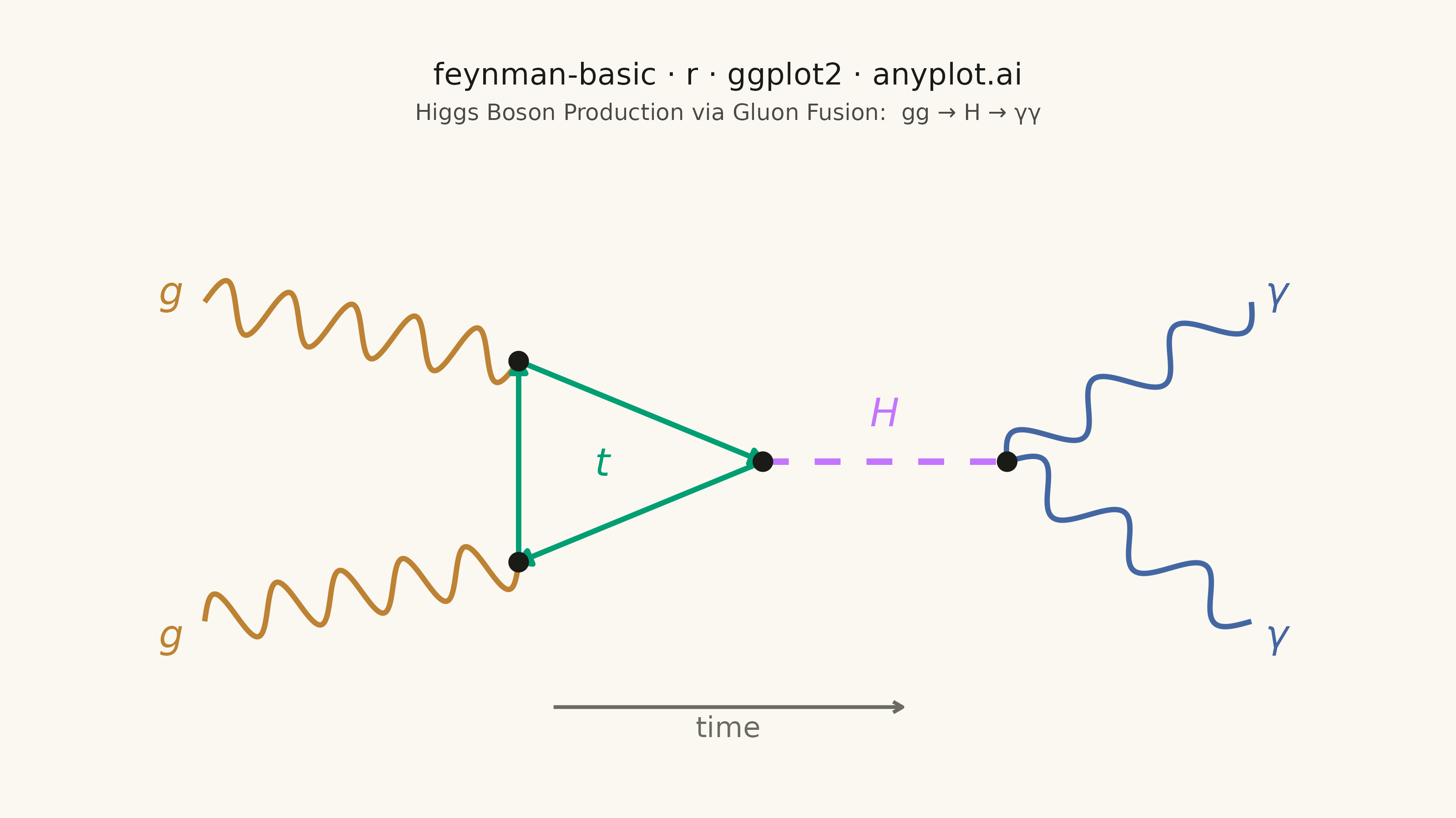
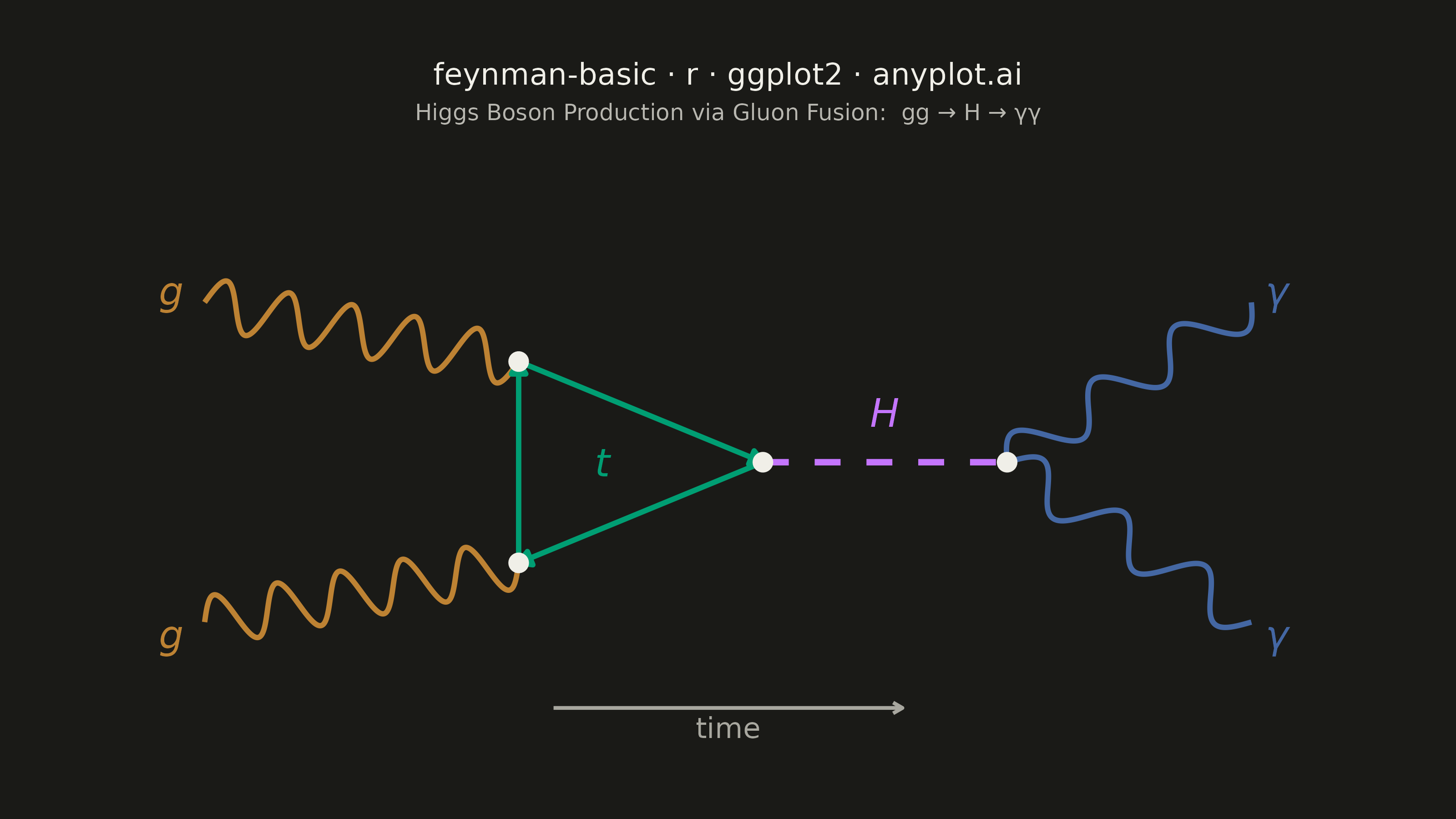
A Feynman diagram visualizes interactions between subatomic particles in quantum field theory. Different line styles represent different particle types: straight lines for fermions (electrons, quarks), wavy lines for photons, curly/looped lines for gluons, and dashed lines for scalar bosons (e.g., Higgs). Lines meet at vertices representing interaction points. Invented by Richard Feynman, these diagrams are both a computational tool and a cultural icon of modern physics.
#' anyplot.ai
#' feynman-basic: Feynman Diagram for Particle Interactions
#' Library: ggplot2 3.5.1 | R 4.4.1
#' Quality: 93/100 | Created: 2026-06-03

library(ggplot2)
library(dplyr)
library(tibble)
library(ragg)

# --- Theme tokens -----------------------------------------------------------
THEME       <- Sys.getenv("ANYPLOT_THEME", "light")
PAGE_BG     <- if (THEME == "light") "#FAF8F1" else "#1A1A17"
INK         <- if (THEME == "light") "#1A1A17" else "#F0EFE8"
INK_SOFT    <- if (THEME == "light") "#4A4A44" else "#B8B7B0"
INK_MUTED   <- if (THEME == "light") "#6B6A63" else "#A8A79F"

# Imprint palette — semantic assignments for all 4 particle types
COL_FERMION <- "#009E73"  # pos 1 — quarks/fermions (green)
COL_BOSON   <- "#C475FD"  # pos 2 — scalar Higgs boson (lavender)
COL_PHOTON  <- "#4467A3"  # pos 3 — photons (blue, EM radiation)
COL_GLUON   <- "#BD8233"  # pos 4 — gluons (ochre, QCD)

# --- Helper: wavy photon line (sinusoidal, perpendicular to path) -----------
wavy_line <- function(x0, y0, x1, y1, n_waves = 3, amplitude = 0.35, n_pts = 300) {
  t   <- seq(0, 1, length.out = n_pts)
  dx  <- x1 - x0;  dy  <- y1 - y0
  len <- sqrt(dx^2 + dy^2)
  px  <- -dy / len; py  <-  dx / len
  wave <- amplitude * sin(n_waves * 2 * pi * t)
  tibble(x = x0 + t * dx + wave * px,
         y = y0 + t * dy + wave * py)
}

# --- Helper: curly gluon line (higher-frequency sinusoid — visually curlier) -
gluon_line <- function(x0, y0, x1, y1, n_loops = 6, amplitude = 0.42, n_pts = 500) {
  t   <- seq(0, 1, length.out = n_pts)
  dx  <- x1 - x0;  dy  <- y1 - y0
  len <- sqrt(dx^2 + dy^2)
  px  <- -dy / len; py  <-  dx / len
  curl <- amplitude * sin(n_loops * 2 * pi * t)
  tibble(x = x0 + t * dx + curl * px,
         y = y0 + t * dy + curl * py)
}

# --- Diagram: gg -> H -> gamma gamma (Higgs via gluon fusion) ---------------
# Coordinate space: x in [0, 16], y in [0, 9]  (16:9 aspect ratio)
#
# Process: two gluons (curly) fuse via a top-quark loop (fermion triangle)
# producing a Higgs boson (dashed) that decays to two photons (wavy).
# All 4 Feynman line types are shown.

VT <- c(5.0, 6.2)   # top gluon-quark vertex
VB <- c(5.0, 2.8)   # bottom gluon-quark vertex
VR <- c(8.5, 4.5)   # quark-loop / Higgs emission vertex
VH <- c(12.0, 4.5)  # Higgs decay vertex (H -> gamma gamma)

# Gluon lines (curly, ochre) — incoming from left
gluons <- bind_rows(
  gluon_line(0.5, 7.2, VT[1], VT[2], n_loops = 5) |> mutate(group = "g_top"),
  gluon_line(0.5, 1.8, VB[1], VB[2], n_loops = 5) |> mutate(group = "g_bot")
)

# Fermion (top quark) loop — triangle: VT -> VR -> VB -> VT
quark_loop <- tibble(
  x    = c(VT[1], VR[1], VB[1]),
  y    = c(VT[2], VR[2], VB[2]),
  xend = c(VR[1], VB[1], VT[1]),
  yend = c(VR[2], VB[2], VT[2])
)

# Higgs propagator (dashed, lavender) — VR to VH
higgs_seg <- tibble(x = VR[1], y = VR[2], xend = VH[1], yend = VH[2])

# Photon lines (wavy, blue) — Higgs decays to two photons
photons <- bind_rows(
  wavy_line(VH[1], VH[2], 15.5, 7.2, n_waves = 3) |> mutate(group = "gamma_top"),
  wavy_line(VH[1], VH[2], 15.5, 1.8, n_waves = 3) |> mutate(group = "gamma_bot")
)

# All four interaction vertices
vertices <- tibble(
  x = c(VT[1], VB[1], VR[1], VH[1]),
  y = c(VT[2], VB[2], VR[2], VH[2])
)

# Particle labels — colored to match their line type
labels_df <- tibble(
  x     = c(0.2,      0.2,      10.25,    15.7,     15.7,     6.2),
  y     = c(7.4,      1.6,      5.1,      7.4,      1.6,      4.5),
  label = c("g",      "g",      "H",      "γ", "γ", "t"),
  hjust = c(1.0,      1.0,      0.5,      0.0,      0.0,      0.5),
  vjust = c(0.5,      0.5,      0.0,      0.5,      0.5,      0.5),
  col   = c(COL_GLUON, COL_GLUON, COL_BOSON, COL_PHOTON, COL_PHOTON, COL_FERMION)
)

# --- Title ------------------------------------------------------------------
plot_title    <- "feynman-basic · r · ggplot2 · anyplot.ai"
plot_subtitle <- "Higgs Boson Production via Gluon Fusion:  gg → H → γγ"

# --- Build plot -------------------------------------------------------------
p <- ggplot() +
  # Gluon curly lines (ochre) — two incoming gluons
  geom_path(data = gluons, aes(x = x, y = y, group = group),
            color = COL_GLUON, linewidth = 1.0) +
  # Top-quark fermion loop — triangle with directional arrows (green)
  geom_segment(data = quark_loop,
               aes(x = x, y = y, xend = xend, yend = yend),
               color = COL_FERMION, linewidth = 1.0,
               arrow = arrow(length = unit(0.20, "cm"), type = "closed", ends = "last")) +
  # Higgs scalar propagator (lavender dashed)
  geom_segment(data = higgs_seg, aes(x = x, y = y, xend = xend, yend = yend),
               color = COL_BOSON, linewidth = 1.2, linetype = "dashed") +
  # Photon wavy lines (blue) — two outgoing photons from H decay
  geom_path(data = photons, aes(x = x, y = y, group = group),
            color = COL_PHOTON, linewidth = 1.0) +
  # Interaction vertex dots (theme-adaptive INK color)
  geom_point(data = vertices, aes(x = x, y = y),
             color = INK, size = 3.5, shape = 16) +
  # Particle labels — colored italic, using scale_color_identity()
  geom_text(data = labels_df,
            aes(x = x, y = y, label = label,
                hjust = hjust, vjust = vjust, color = col),
            size = 5.5, fontface = "italic") +
  scale_color_identity() +
  # Time direction arrow at bottom
  annotate("segment", x = 5.5, xend = 10.5, y = 0.35, yend = 0.35,
           color = INK_MUTED, linewidth = 0.7,
           arrow = arrow(length = unit(0.15, "cm"), type = "open")) +
  annotate("text", x = 8.0, y = 0.02, label = "time",
           color = INK_MUTED, size = 4.0, hjust = 0.5) +
  coord_cartesian(xlim = c(-0.5, 16.5), ylim = c(-0.2, 9.3)) +
  labs(title = plot_title, subtitle = plot_subtitle) +
  theme_void() +
  theme(
    plot.background = element_rect(fill = PAGE_BG, color = PAGE_BG),
    plot.title      = element_text(color = INK,      size = 12, hjust = 0.5,
                                   margin = margin(t = 15, b = 5)),
    plot.subtitle   = element_text(color = INK_SOFT, size = 9,  hjust = 0.5,
                                   margin = margin(b = 10)),
    plot.margin     = margin(t = 10, r = 30, b = 20, l = 30)
  )

# --- Save -------------------------------------------------------------------
ggsave(
  filename = sprintf("plot-%s.png", THEME),
  plot     = p,
  device   = ragg::agg_png,
  width    = 8,
  height   = 4.5,
  units    = "in",
  dpi      = 400
)
Runnable source as JSON, for any HTTP client: https://api.anyplot.ai/specs/feynman-basic/ggplot2/code. Any spec id and library id listed in llms-full.txt fit the same URL shape; every URL below is complete and callable.
{
  "spec_id": "feynman-basic",
  "language": "r",
  "library": "ggplot2",
  "page": "https://anyplot.ai/feynman-basic/r/ggplot2",
  "hub": "https://anyplot.ai/feynman-basic",
  "code_json": "https://api.anyplot.ai/specs/feynman-basic/ggplot2/code",
  "spec_json": "https://api.anyplot.ai/specs/feynman-basic",
  "render_light_png": "https://storage.googleapis.com/anyplot-images/plots/feynman-basic/r/ggplot2/plot-light.png",
  "render_dark_png": "https://storage.googleapis.com/anyplot-images/plots/feynman-basic/r/ggplot2/plot-dark.png",
  "quality_score": 93.0,
  "license": "MIT",
  "guide": "https://anyplot.ai/llms.txt"
}
Part of Feynman Diagram for Particle Interactions on anyplot.ai.