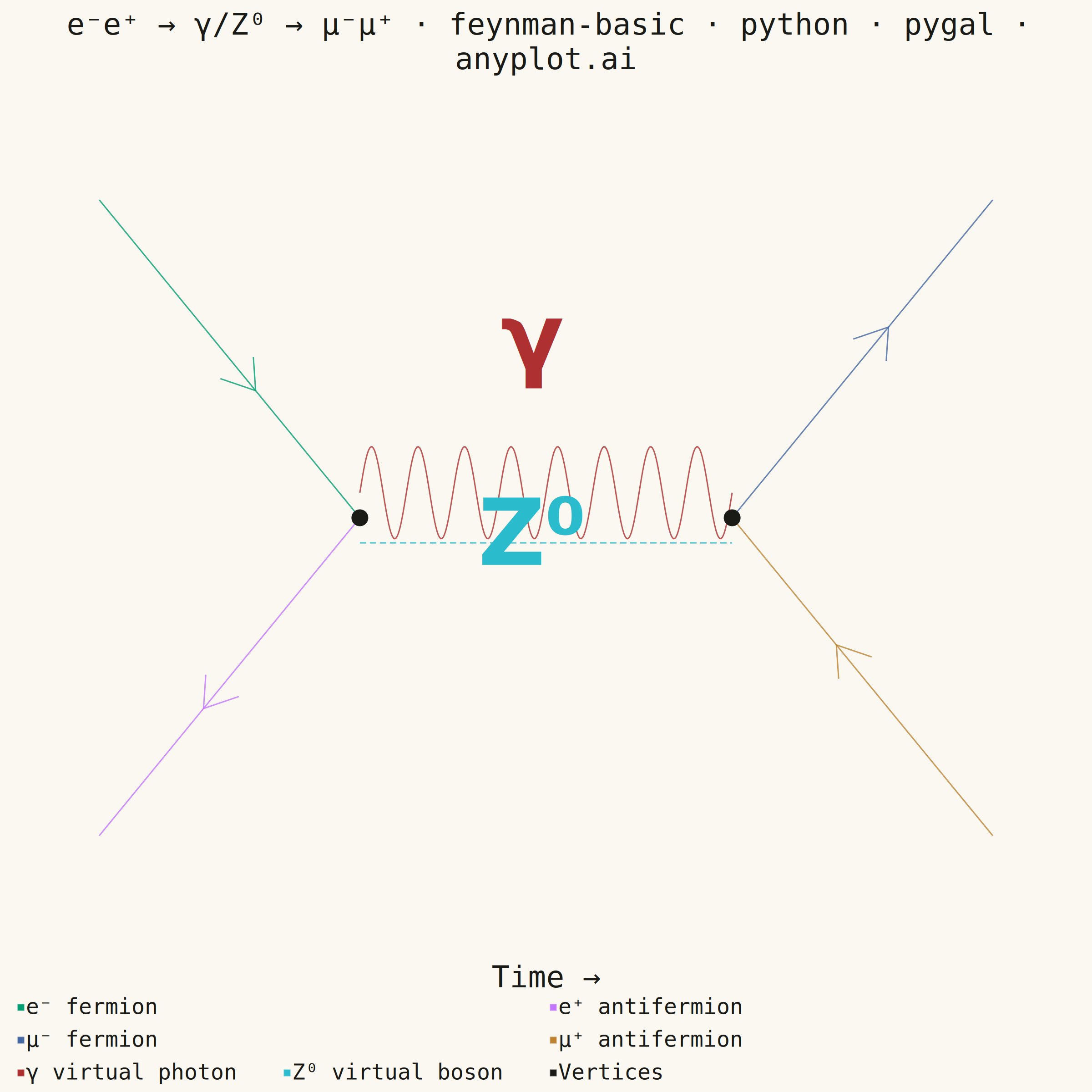
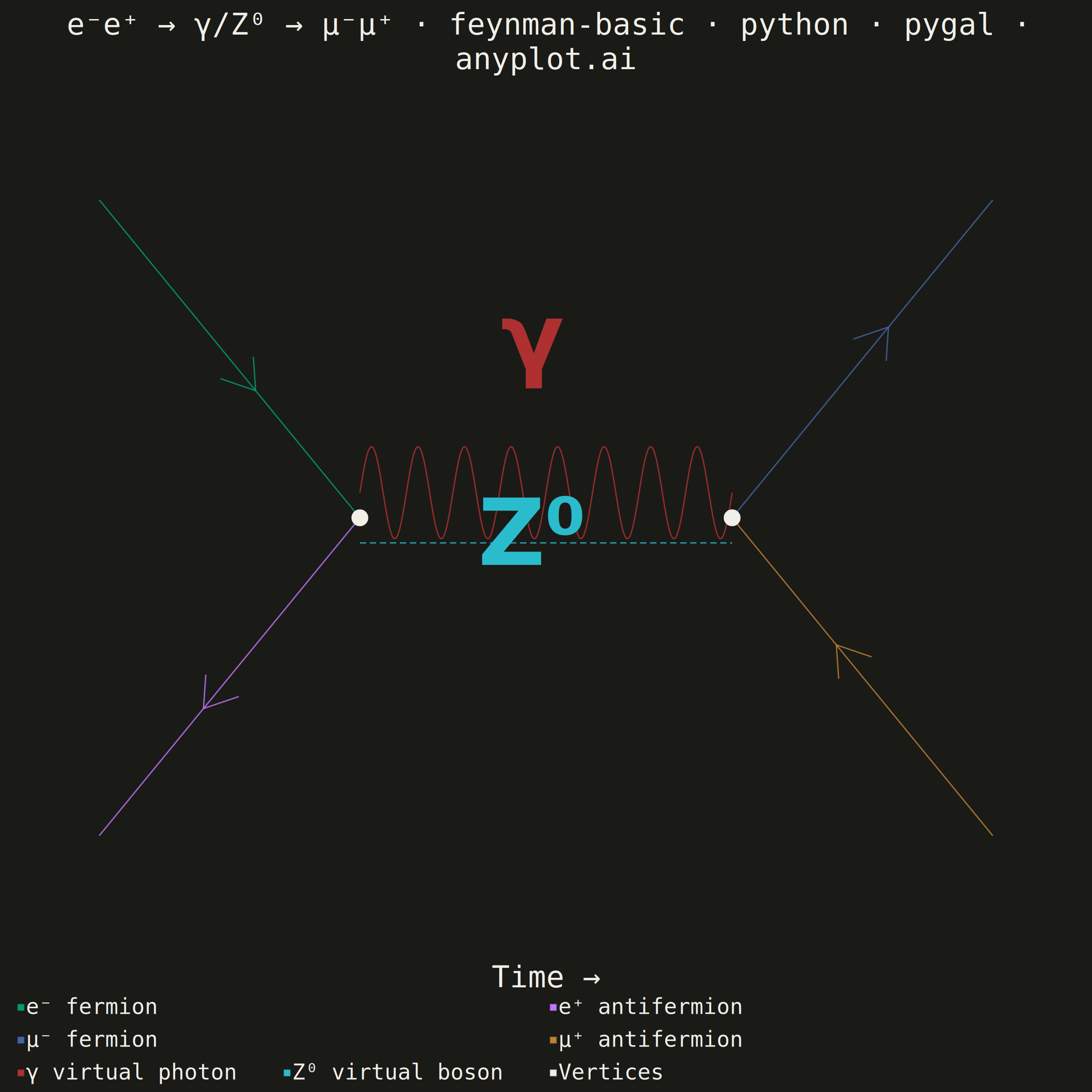
A Feynman diagram visualizes interactions between subatomic particles in quantum field theory. Different line styles represent different particle types: straight lines for fermions (electrons, quarks), wavy lines for photons, curly/looped lines for gluons, and dashed lines for scalar bosons (e.g., Higgs). Lines meet at vertices representing interaction points. Invented by Richard Feynman, these diagrams are both a computational tool and a cultural icon of modern physics.
""" anyplot.ai
feynman-basic: Feynman Diagram for Particle Interactions
Library: pygal 3.1.0 | Python 3.13.13
Quality: 82/100 | Updated: 2026-06-03
"""

import os
import re
import sys as _sys


# Remove this file's directory from sys.path so 'import pygal' finds the installed
# package instead of this file (which shares its name with the library).
_this_dir = os.path.dirname(os.path.abspath(__file__))
_sys.path[:] = [p for p in _sys.path if os.path.abspath(p or ".") != _this_dir]
del _this_dir, _sys

import numpy as np
import pygal
from pygal.style import Style


# Theme tokens — Imprint palette, theme-adaptive chrome
THEME = os.getenv("ANYPLOT_THEME", "light")
PAGE_BG = "#FAF8F1" if THEME == "light" else "#1A1A17"
INK = "#1A1A17" if THEME == "light" else "#F0EFE8"
INK_MUTED = "#6B6A63" if THEME == "light" else "#A8A79F"

# Imprint palette — doubled entries for arrowhead series to share fermion color
PALETTE = (
    "#009E73",
    "#009E73",  # e⁻ fermion + arrowhead  (Imprint #1)
    "#C475FD",
    "#C475FD",  # e⁺ antifermion + arrowhead  (Imprint #2)
    "#4467A3",
    "#4467A3",  # μ⁻ fermion + arrowhead  (Imprint #3)
    "#BD8233",
    "#BD8233",  # μ⁺ antifermion + arrowhead  (Imprint #4)
    "#AE3030",  # γ virtual photon  (Imprint #5)
    "#2ABCCD",  # Z⁰ virtual boson  (Imprint #6)
    INK,  # vertex markers
)

# Data — e⁻e⁺ → γ / Z⁰ → μ⁻μ⁺  (QED + electroweak s-channel annihilation)
v1 = (3.0, 5.0)  # annihilation vertex
v2 = (7.0, 5.0)  # pair creation vertex

e_minus_ep = (0.2, 8.8)
e_plus_ep = (0.2, 1.2)
mu_minus_ep = (9.8, 8.8)
mu_plus_ep = (9.8, 1.2)

# Fermion propagator lines (2-point series)
e_minus_line = [
    {"value": e_minus_ep, "label": "e⁻ incoming fermion"},
    {"value": v1, "label": "Vertex 1 — annihilation"},
]
e_plus_line = [
    {"value": e_plus_ep, "label": "e⁺ incoming antifermion"},
    {"value": v1, "label": "Vertex 1 — annihilation"},
]
mu_minus_line = [
    {"value": v2, "label": "Vertex 2 — pair creation"},
    {"value": mu_minus_ep, "label": "μ⁻ outgoing fermion"},
]
mu_plus_line = [
    {"value": v2, "label": "Vertex 2 — pair creation"},
    {"value": mu_plus_ep, "label": "μ⁺ outgoing antifermion"},
]

# Arrowhead V-shapes — inline numpy computation per fermion line
# Convention: particle flows left→right (forward in time), antiparticle right→left
_frac, _sz, _hw = 0.60, 0.34, 0.22  # arrow position, size, half-width

# e⁻ arrowhead: (e_minus_ep → v1), particle flows forward
_p1, _p2 = np.array(e_minus_ep), np.array(v1)
_d = _p2 - _p1
_l = float(np.linalg.norm(_d))
_u = _d / _l
_q = np.array([-_u[1], _u[0]])
_tp = _p1 + _frac * _d
_bs = _tp - _sz * _u
e_minus_arrow = [
    {"value": (float(_bs[0] + _hw * _q[0]), float(_bs[1] + _hw * _q[1])), "label": "wing"},
    {"value": (float(_tp[0]), float(_tp[1])), "label": "→ tip"},
    {"value": (float(_bs[0] - _hw * _q[0]), float(_bs[1] - _hw * _q[1])), "label": "wing"},
]

# e⁺ arrowhead: (v1 → e_plus_ep), antiparticle flows backward in time
_p1, _p2 = np.array(v1), np.array(e_plus_ep)
_d = _p2 - _p1
_l = float(np.linalg.norm(_d))
_u = _d / _l
_q = np.array([-_u[1], _u[0]])
_tp = _p1 + _frac * _d
_bs = _tp - _sz * _u
e_plus_arrow = [
    {"value": (float(_bs[0] + _hw * _q[0]), float(_bs[1] + _hw * _q[1])), "label": "wing"},
    {"value": (float(_tp[0]), float(_tp[1])), "label": "← tip"},
    {"value": (float(_bs[0] - _hw * _q[0]), float(_bs[1] - _hw * _q[1])), "label": "wing"},
]

# μ⁻ arrowhead: (v2 → mu_minus_ep), particle flows forward
_p1, _p2 = np.array(v2), np.array(mu_minus_ep)
_d = _p2 - _p1
_l = float(np.linalg.norm(_d))
_u = _d / _l
_q = np.array([-_u[1], _u[0]])
_tp = _p1 + _frac * _d
_bs = _tp - _sz * _u
mu_minus_arrow = [
    {"value": (float(_bs[0] + _hw * _q[0]), float(_bs[1] + _hw * _q[1])), "label": "wing"},
    {"value": (float(_tp[0]), float(_tp[1])), "label": "→ tip"},
    {"value": (float(_bs[0] - _hw * _q[0]), float(_bs[1] - _hw * _q[1])), "label": "wing"},
]

# μ⁺ arrowhead: (mu_plus_ep → v2), antiparticle flows backward in time
_p1, _p2 = np.array(mu_plus_ep), np.array(v2)
_d = _p2 - _p1
_l = float(np.linalg.norm(_d))
_u = _d / _l
_q = np.array([-_u[1], _u[0]])
_tp = _p1 + _frac * _d
_bs = _tp - _sz * _u
mu_plus_arrow = [
    {"value": (float(_bs[0] + _hw * _q[0]), float(_bs[1] + _hw * _q[1])), "label": "wing"},
    {"value": (float(_tp[0]), float(_tp[1])), "label": "← tip"},
    {"value": (float(_bs[0] - _hw * _q[0]), float(_bs[1] - _hw * _q[1])), "label": "wing"},
]

# Photon propagator — sinusoidal wavy path slightly above centre
t = np.linspace(0, 1, 300)
photon_x = v1[0] + t * (v2[0] - v1[0])
photon_y = 5.3 + 0.55 * np.sin(t * 16 * np.pi)
photon_line = [
    {"value": (float(x), float(y)), "label": "γ virtual photon"} for x, y in zip(photon_x, photon_y, strict=True)
]

# Z⁰ boson propagator — dashed line slightly below centre (electroweak mediator)
t_z = np.linspace(0, 1, 200)
z_x = v1[0] + t_z * (v2[0] - v1[0])
z_y = np.full(200, 4.7)
z_line = [{"value": (float(x), float(y)), "label": "Z⁰ virtual boson"} for x, y in zip(z_x, z_y, strict=True)]

# Vertex markers — interaction points
vertex_points = [
    {"value": v1, "label": "Vertex 1 — e⁻e⁺ annihilation"},
    {"value": v2, "label": "Vertex 2 — μ⁻μ⁺ pair creation"},
]

# Style — Imprint palette, theme-adaptive chrome, 2400×2400 canvas sizing
title = "e⁻e⁺ → γ/Z⁰ → μ⁻μ⁺ · feynman-basic · python · pygal · anyplot.ai"
_n = len(title)
_title_fs = round(66 * 67 / _n) if _n > 67 else 66

custom_style = Style(
    background=PAGE_BG,
    plot_background=PAGE_BG,
    foreground=INK,
    foreground_strong=INK,
    foreground_subtle=INK_MUTED,
    colors=PALETTE,
    opacity=1.0,
    opacity_hover=0.9,
    title_font_size=_title_fs,
    label_font_size=56,
    major_label_font_size=44,
    legend_font_size=48,
    value_font_size=36,
    stroke_width=3.0,
    legend_box_size=30,
)

# Chart — square canvas for symmetric Feynman diagram
chart = pygal.XY(
    width=2400,
    height=2400,
    style=custom_style,
    title=title,
    show_x_guides=False,
    show_y_guides=False,
    show_x_labels=False,
    show_y_labels=False,
    x_title="Time →",
    y_title="",
    show_legend=True,
    legend_at_bottom=True,
    legend_at_bottom_columns=4,
    stroke=True,
    show_dots=False,
    print_values=False,
    margin_top=30,
    margin_bottom=100,
    margin_left=30,
    margin_right=30,
    range=(0.0, 10.0),
    xrange=(-0.5, 10.5),
)

# Fermion lines + direction arrowheads (interleaved to match palette)
chart.add("e⁻ fermion", e_minus_line, stroke_width=7)
chart.add("e⁻ (→)", e_minus_arrow, stroke_width=6, show_dots=False)
chart.add("e⁺ antifermion", e_plus_line, stroke_width=7)
chart.add("e⁺ (←)", e_plus_arrow, stroke_width=6, show_dots=False)
chart.add("μ⁻ fermion", mu_minus_line, stroke_width=7)
chart.add("μ⁻ (→)", mu_minus_arrow, stroke_width=6, show_dots=False)
chart.add("μ⁺ antifermion", mu_plus_line, stroke_width=7)
chart.add("μ⁺ (←)", mu_plus_arrow, stroke_width=6, show_dots=False)

# Propagators
chart.add("γ virtual photon", photon_line, stroke_width=5)
chart.add("Z⁰ virtual boson", z_line, stroke_width=4, stroke_style={"dasharray": "14 8"})

# Vertex markers
chart.add("Vertices", vertex_points, stroke=False, show_dots=True, dots_size=18)


# Post-process SVG for PNG: remove arrowhead legend entries and add on-diagram
# particle labels for γ and Z⁰ propagators.
# Series 1,3,5,7 (0-indexed) are the arrowhead helpers — hidden from legend in PNG.
# Vertex circles (dots_size=18) anchor the coordinate transform for label placement.
def _process_svg_for_png(svg_bytes):
    svg = svg_bytes.decode("utf-8")

    # Remove arrowhead legend entries by series id
    for idx in (1, 3, 5, 7):
        svg = re.sub(rf'<g\b[^>]*\bid="activate-serie-{idx}"[^>]*>[\s\S]*?</g>', "", svg)

    # Find vertex-marker circles (dots_size=18 → r≈18 in SVG)
    vertex_pts = []
    for c in re.findall(r"<circle\b[^>]+>", svg, flags=re.IGNORECASE):
        cx_m = re.search(r"\bcx=[\"']([^\"']+)[\"']", c)
        cy_m = re.search(r"\bcy=[\"']([^\"']+)[\"']", c)
        r_m = re.search(r"\br=[\"']([^\"']+)[\"']", c)
        if cx_m and cy_m and r_m and 14 < float(r_m.group(1)) < 26:
            vertex_pts.append((float(cx_m.group(1)), float(cy_m.group(1))))

    if len(vertex_pts) >= 2:
        vertex_pts.sort(key=lambda p: p[0])
        sv1, sv2 = vertex_pts[0], vertex_pts[1]  # SVG px for v1=(3,5), v2=(7,5)
        # x_scale: SVG pixels per data unit (derived from known Δx = 4 data units)
        x_scale = (sv2[0] - sv1[0]) / (7.0 - 3.0)
        # y_scale approximated as x_scale (square canvas, similar x/y data spans)
        y_scale = x_scale
        mid_sx = sv1[0] + 2.0 * x_scale  # data x=5.0 → midpoint
        mid_sy = sv1[1]  # sv1[1] corresponds to data y=5.0
        font_px = max(60, int(x_scale * 1.0))
        g_sy = mid_sy - 1.05 * y_scale  # above wavy γ line
        z_sy = mid_sy + 1.05 * y_scale  # below dashed Z⁰ line
        svg = svg.replace(
            "</svg>",
            f'<text x="{mid_sx:.0f}" y="{g_sy:.0f}" font-family="sans-serif" '
            f'font-size="{font_px}" font-weight="bold" fill="#AE3030" '
            f'text-anchor="middle" dominant-baseline="central">γ</text>\n'
            f'<text x="{mid_sx:.0f}" y="{z_sy:.0f}" font-family="sans-serif" '
            f'font-size="{font_px}" font-weight="bold" fill="#2ABCCD" '
            f'text-anchor="middle" dominant-baseline="central">Z⁰</text>\n'
            "</svg>",
            1,
        )

    return svg.encode("utf-8")


from cairosvg import svg2png


svg_bytes = chart.render()
svg2png(bytestring=_process_svg_for_png(svg_bytes), write_to=f"plot-{THEME}.png", output_width=2400, output_height=2400)
with open(f"plot-{THEME}.html", "wb") as f:
    f.write(svg_bytes)
Runnable source as JSON, for any HTTP client: https://api.anyplot.ai/specs/feynman-basic/pygal/code. Any spec id and library id listed in llms-full.txt fit the same URL shape; every URL below is complete and callable.
{
  "spec_id": "feynman-basic",
  "language": "python",
  "library": "pygal",
  "page": "https://anyplot.ai/feynman-basic/python/pygal",
  "hub": "https://anyplot.ai/feynman-basic",
  "code_json": "https://api.anyplot.ai/specs/feynman-basic/pygal/code",
  "spec_json": "https://api.anyplot.ai/specs/feynman-basic",
  "render_light_png": "https://storage.googleapis.com/anyplot-images/plots/feynman-basic/python/pygal/plot-light.png",
  "render_dark_png": "https://storage.googleapis.com/anyplot-images/plots/feynman-basic/python/pygal/plot-dark.png",
  "interactive_light_html": "https://storage.googleapis.com/anyplot-images/plots/feynman-basic/python/pygal/plot-light.html",
  "interactive_dark_html": "https://storage.googleapis.com/anyplot-images/plots/feynman-basic/python/pygal/plot-dark.html",
  "quality_score": 82.0,
  "license": "MIT",
  "guide": "https://anyplot.ai/llms.txt"
}
Part of Feynman Diagram for Particle Interactions on anyplot.ai.