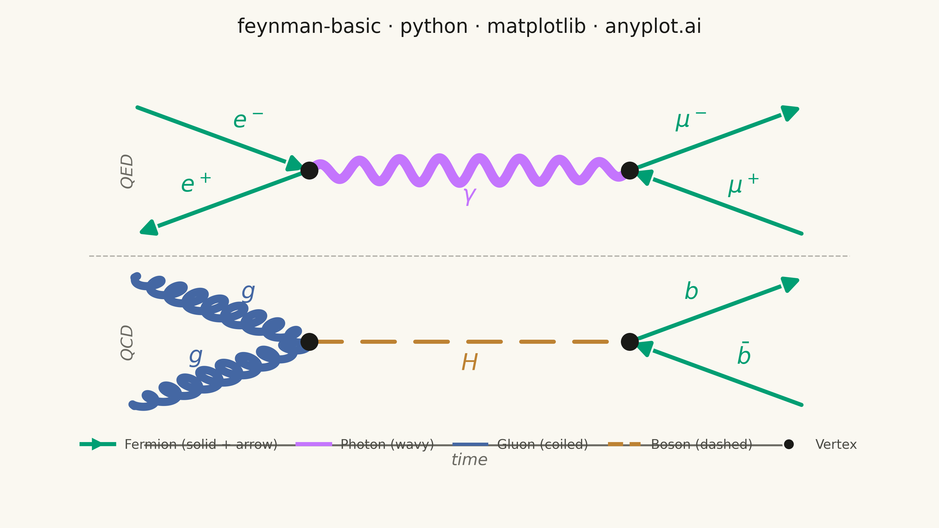
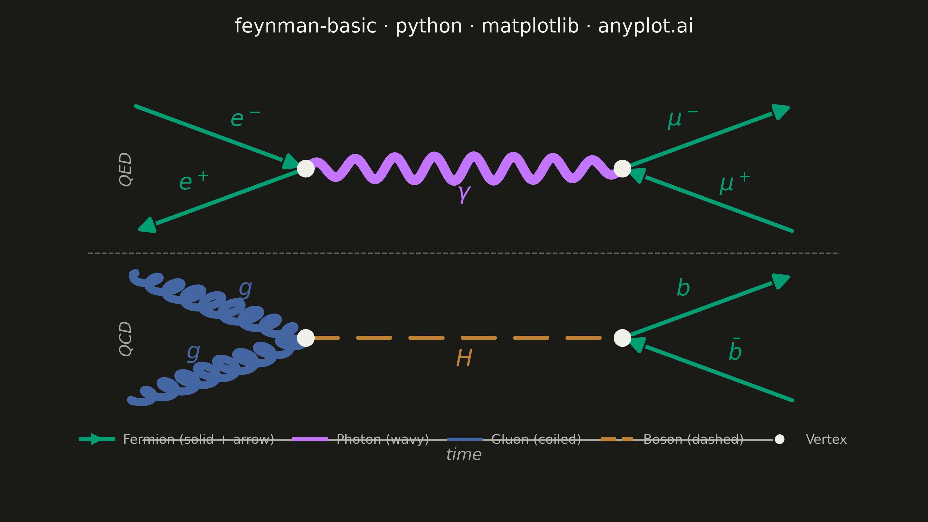
A Feynman diagram visualizes interactions between subatomic particles in quantum field theory. Different line styles represent different particle types: straight lines for fermions (electrons, quarks), wavy lines for photons, curly/looped lines for gluons, and dashed lines for scalar bosons (e.g., Higgs). Lines meet at vertices representing interaction points. Invented by Richard Feynman, these diagrams are both a computational tool and a cultural icon of modern physics.
""" anyplot.ai
feynman-basic: Feynman Diagram for Particle Interactions
Library: matplotlib 3.10.9 | Python 3.13.13
Quality: 91/100 | Updated: 2026-06-03
"""

import os

import matplotlib.patheffects as pe
import matplotlib.pyplot as plt
import numpy as np
from matplotlib.lines import Line2D
from matplotlib.patches import FancyArrowPatch


THEME = os.getenv("ANYPLOT_THEME", "light")

# Theme-adaptive chrome — Imprint palette
PAGE_BG = "#FAF8F1" if THEME == "light" else "#1A1A17"
INK = "#1A1A17" if THEME == "light" else "#F0EFE8"
INK_SOFT = "#4A4A44" if THEME == "light" else "#B8B7B0"
INK_MUTED = "#6B6A63" if THEME == "light" else "#A8A79F"

# Imprint categorical palette — particle types (positions 1–4)
FERMION_COLOR = "#009E73"  # pos 1: brand green
PHOTON_COLOR = "#C475FD"  # pos 2: lavender
GLUON_COLOR = "#4467A3"  # pos 3: blue
BOSON_COLOR = "#BD8233"  # pos 4: ochre

# Two-process layout: top QED (e+e- annihilation), bottom QCD (gg -> H)
vertices = {"v1": (0.28, 0.74), "v2": (0.72, 0.74), "v3": (0.28, 0.26), "v4": (0.72, 0.26)}

propagators = [
    # QED: e-e+ -> gamma -> mu-mu+
    {"from": (0.04, 0.92), "to": "v1", "type": "fermion", "label": r"$e^-$", "arrow_fwd": True},
    {"from": (0.04, 0.56), "to": "v1", "type": "fermion", "label": r"$e^+$", "arrow_fwd": False},
    {"from": "v1", "to": "v2", "type": "photon", "label": r"$\gamma$"},
    {"from": "v2", "to": (0.96, 0.92), "type": "fermion", "label": r"$\mu^-$", "arrow_fwd": True},
    {"from": "v2", "to": (0.96, 0.56), "type": "fermion", "label": r"$\mu^+$", "arrow_fwd": False},
    # QCD: gg -> H -> bb-bar
    {"from": (0.04, 0.44), "to": "v3", "type": "gluon", "label": r"$g$"},
    {"from": (0.04, 0.08), "to": "v3", "type": "gluon", "label": r"$g$"},
    {"from": "v3", "to": "v4", "type": "boson", "label": r"$H$"},
    {"from": "v4", "to": (0.96, 0.44), "type": "fermion", "label": r"$b$", "arrow_fwd": True},
    {"from": "v4", "to": (0.96, 0.08), "type": "fermion", "label": r"$\bar{b}$", "arrow_fwd": False},
]

# Canvas: landscape 3200×1800 px (figsize=(8, 4.5), dpi=400)
fig, ax = plt.subplots(figsize=(8, 4.5), dpi=400, facecolor=PAGE_BG)
ax.set_facecolor(PAGE_BG)
ax.set_xlim(-0.08, 1.08)
ax.set_ylim(-0.08, 1.08)

for prop in propagators:
    start = vertices[prop["from"]] if isinstance(prop["from"], str) else prop["from"]
    end = vertices[prop["to"]] if isinstance(prop["to"], str) else prop["to"]
    sx, sy = start
    ex, ey = end
    mx, my = (sx + ex) / 2, (sy + ey) / 2
    dx, dy = ex - sx, ey - sy
    length = np.sqrt(dx**2 + dy**2)
    ux, uy = dx / length, dy / length
    px, py = -uy, ux  # perpendicular unit vector

    if prop["type"] == "fermion":
        arrow_fwd = prop.get("arrow_fwd", True)
        # FancyArrowPatch: direct matplotlib Patch API for arrow rendering
        arrow = FancyArrowPatch(
            posA=(sx, sy) if arrow_fwd else (ex, ey),
            posB=(ex, ey) if arrow_fwd else (sx, sy),
            arrowstyle="-|>",
            color=FERMION_COLOR,
            linewidth=2.5,
            mutation_scale=20,
            transform=ax.transData,
            zorder=3,
        )
        # patheffects: background-color halo separates the arrow from any crossing lines
        arrow.set_path_effects([pe.withStroke(linewidth=5, foreground=PAGE_BG)])
        ax.add_patch(arrow)
        ax.text(
            mx + px * 0.06,
            my + py * 0.06,
            prop["label"],
            fontsize=14,
            ha="center",
            va="center",
            color=FERMION_COLOR,
            fontweight="bold",
        )

    elif prop["type"] == "photon":
        t = np.linspace(0, 1, 500)
        wave = 0.035 * np.sin(2 * np.pi * 8 * t) * np.sin(np.pi * t) ** 0.3
        (line,) = ax.plot(
            sx + t * dx + wave * px, sy + t * dy + wave * py, color=PHOTON_COLOR, lw=2.5, solid_capstyle="round"
        )
        # patheffects: wider same-color stroke gives the wave a luminous, glowing appearance
        line.set_path_effects([pe.withStroke(linewidth=6, foreground=PHOTON_COLOR)])
        ax.text(
            mx - px * 0.07,
            my - py * 0.07,
            prop["label"],
            fontsize=14,
            ha="center",
            va="center",
            color=PHOTON_COLOR,
            fontweight="bold",
        )

    elif prop["type"] == "gluon":
        t = np.linspace(0, 1, 3000)
        phase = 2 * np.pi * 9 * t
        envelope = np.sin(np.pi * t) ** 0.4
        along_mod = 0.025 * 0.7 * np.sin(phase) * envelope
        perp_disp = 0.025 * np.cos(phase) * envelope
        (line,) = ax.plot(
            sx + t * dx - along_mod * ux + perp_disp * px,
            sy + t * dy - along_mod * uy + perp_disp * py,
            color=GLUON_COLOR,
            lw=2.0,
            solid_capstyle="round",
        )
        # patheffects: wider stroke gives the coil visual weight consistent with the photon glow
        line.set_path_effects([pe.withStroke(linewidth=5, foreground=GLUON_COLOR)])
        ax.text(
            mx + px * 0.06,
            my + py * 0.06,
            prop["label"],
            fontsize=14,
            ha="center",
            va="center",
            color=GLUON_COLOR,
            fontweight="bold",
        )

    elif prop["type"] == "boson":
        ax.plot([sx, ex], [sy, ey], color=BOSON_COLOR, lw=2.5, linestyle=(0, (8, 5)), dash_capstyle="round")
        ax.text(
            mx - px * 0.06,
            my - py * 0.06,
            prop["label"],
            fontsize=14,
            ha="center",
            va="center",
            color=BOSON_COLOR,
            fontweight="bold",
        )

# Vertex dots (theme-adaptive ink)
for vx, vy in vertices.values():
    ax.plot(vx, vy, "o", color=INK, markersize=10, zorder=5)

# Separator between QED and QCD processes
ax.axhline(y=0.50, xmin=0.05, xmax=0.95, color=INK_MUTED, lw=0.8, linestyle="--", alpha=0.5)

# Process labels — nudged inward and bumped to 10pt for mobile readability
ax.text(0.02, 0.74, "QED", fontsize=10, ha="left", va="center", color=INK_MUTED, fontstyle="italic", rotation=90)
ax.text(0.02, 0.26, "QCD", fontsize=10, ha="left", va="center", color=INK_MUTED, fontstyle="italic", rotation=90)

# Time arrow (inside axes area, above legend)
ax.annotate("", xy=(0.95, -0.03), xytext=(0.05, -0.03), arrowprops={"arrowstyle": "->", "color": INK_MUTED, "lw": 1.2})
ax.text(0.5, -0.05, "time", fontsize=10, ha="center", va="top", color=INK_MUTED, fontstyle="italic")

# Title (48 chars < 67 threshold — default 12pt)
ax.set_title("feynman-basic · python · matplotlib · anyplot.ai", fontsize=12, fontweight="medium", pad=10, color=INK)
ax.axis("off")

# Legend (frameless for minimal aesthetic)
legend_handles = [
    Line2D(
        [0],
        [0],
        color=FERMION_COLOR,
        lw=2.5,
        marker=">",
        markersize=6,
        markeredgecolor=FERMION_COLOR,
        label="Fermion (solid + arrow)",
    ),
    Line2D([0], [0], color=PHOTON_COLOR, lw=2.5, label="Photon (wavy)"),
    Line2D([0], [0], color=GLUON_COLOR, lw=2.0, label="Gluon (coiled)"),
    Line2D([0], [0], color=BOSON_COLOR, lw=2.5, linestyle="--", label="Boson (dashed)"),
    Line2D([0], [0], marker="o", color=PAGE_BG, markerfacecolor=INK, markersize=7, lw=0, label="Vertex"),
]
leg = ax.legend(
    handles=legend_handles,
    fontsize=8,
    loc="lower center",
    ncol=5,
    frameon=False,
    handlelength=2.5,
    columnspacing=1.5,
    bbox_to_anchor=(0.5, 0.0),
    bbox_transform=ax.transAxes,
)
plt.setp(leg.get_texts(), color=INK_SOFT)

# Reserve bottom 8% of figure for legend below the axes
plt.tight_layout(rect=[0, 0.08, 1, 1])
plt.savefig(f"plot-{THEME}.png", dpi=400, facecolor=PAGE_BG)
Runnable source as JSON, for any HTTP client: https://api.anyplot.ai/specs/feynman-basic/matplotlib/code. Any spec id and library id listed in llms-full.txt fit the same URL shape; every URL below is complete and callable.
{
  "spec_id": "feynman-basic",
  "language": "python",
  "library": "matplotlib",
  "page": "https://anyplot.ai/feynman-basic/python/matplotlib",
  "hub": "https://anyplot.ai/feynman-basic",
  "code_json": "https://api.anyplot.ai/specs/feynman-basic/matplotlib/code",
  "spec_json": "https://api.anyplot.ai/specs/feynman-basic",
  "render_light_png": "https://storage.googleapis.com/anyplot-images/plots/feynman-basic/python/matplotlib/plot-light.png",
  "render_dark_png": "https://storage.googleapis.com/anyplot-images/plots/feynman-basic/python/matplotlib/plot-dark.png",
  "quality_score": 91.0,
  "license": "MIT",
  "guide": "https://anyplot.ai/llms.txt"
}
Part of Feynman Diagram for Particle Interactions on anyplot.ai.