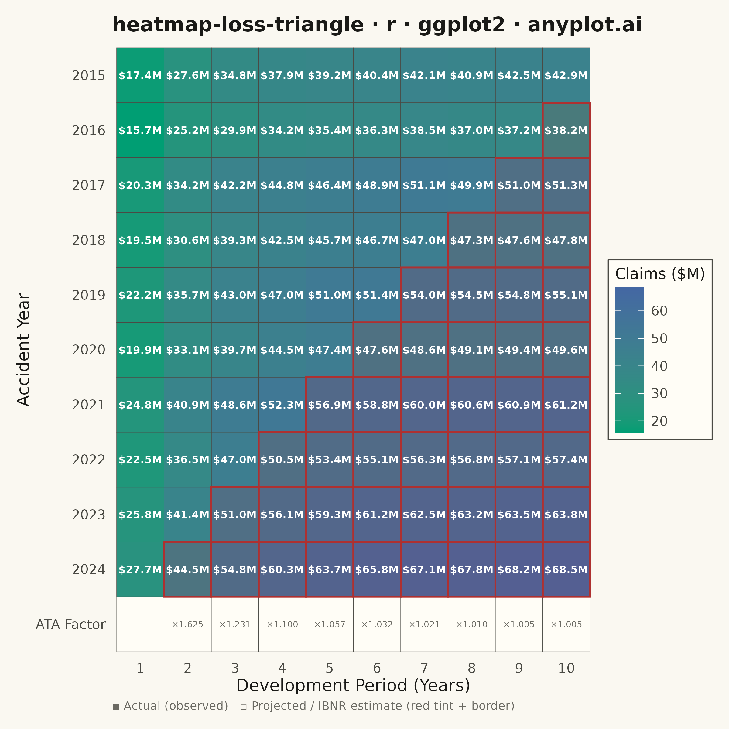
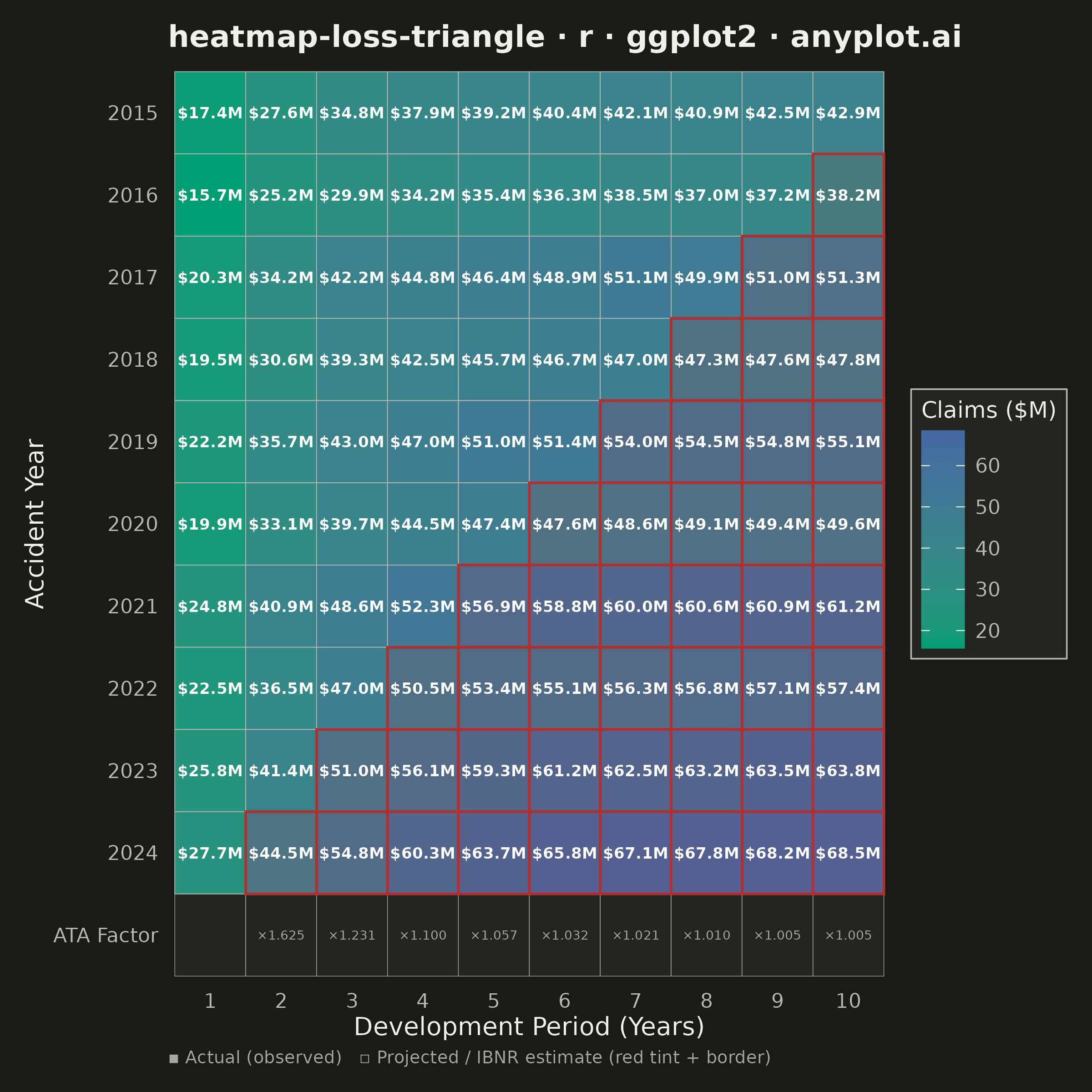
The same plot in 14 other libraries — Python: Altair, Bokeh, lets-plot, Matplotlib, Plotly, plotnine, Pygal, Seaborn; Julia: Makie.jl; JavaScript: Chart.js, D3.js, Apache ECharts, Highcharts, MUI X Charts. Compare all 15 side by side: Actuarial Loss Development Triangle in Python, R, Julia and JavaScript.
A triangular matrix visualization showing cumulative insurance claim payments developing over time. Rows represent accident/origin years, columns represent development periods (e.g., 1-10 years), with the upper-left triangle displaying actual observed cumulative claims and the lower-right triangle showing projected/estimated values (IBNR). This plot is essential for actuarial reserving, enabling analysts to visualize the chain-ladder method and identify development patterns in loss data.
#' anyplot.ai
#' heatmap-loss-triangle: Actuarial Loss Development Triangle
#' Library: ggplot2 3.5.1 | R 4.4.1
#' Quality: 85/100 | Created: 2026-06-03

library(ggplot2)
library(dplyr)
library(scales)
library(ragg)

set.seed(42)

# Theme tokens (Imprint palette, theme-adaptive chrome)
THEME       <- Sys.getenv("ANYPLOT_THEME", "light")
PAGE_BG     <- if (THEME == "light") "#FAF8F1" else "#1A1A17"
ELEVATED_BG <- if (THEME == "light") "#FFFDF6" else "#242420"
INK         <- if (THEME == "light") "#1A1A17" else "#F0EFE8"
INK_SOFT    <- if (THEME == "light") "#4A4A44" else "#B8B7B0"
INK_MUTED   <- if (THEME == "light") "#6B6A63" else "#A8A79F"

# Data: actuarial loss development triangle (chain-ladder method)
accident_years <- 2015:2024
dev_periods    <- 1:10

# Cumulative percent of ultimate paid by development period
pct_paid <- c(0.40, 0.65, 0.80, 0.88, 0.93, 0.96, 0.98, 0.990, 0.995, 1.000)

# Ultimate claims per accident year (in $M)
ultimates <- c(42.5, 38.2, 51.3, 47.8, 55.1, 49.6, 61.2, 57.4, 63.8, 68.5)

# Age-to-age development factors (period p -> period p+1)
ata_factors <- pct_paid[2:10] / pct_paid[1:9]

# y-axis levels: accident years + ATA row at bottom
y_levels <- c(as.character(accident_years), "ATA Factor")
y_limits <- c("ATA Factor", rev(as.character(accident_years)))

# Build full 10 x 10 triangle grid
df <- expand.grid(
  accident_year = accident_years,
  dev_period    = dev_periods,
  stringsAsFactors = FALSE
) %>%
  mutate(
    ay_idx     = accident_year - 2014L,
    is_actual  = dev_period <= (11L - ay_idx),
    cumulative = ultimates[ay_idx] * pct_paid[dev_period],
    cumulative = ifelse(
      is_actual,
      round(cumulative * runif(n(), 0.97, 1.03), 1),
      round(cumulative, 1)
    ),
    label   = sprintf("$%.1fM", cumulative),
    dev_fac = factor(dev_period, levels = 1:10),
    acc_fac = factor(as.character(accident_year), levels = y_levels)
  )

df_proj <- filter(df, !is_actual)

# ATA factor row: background tiles and text annotations
df_ata_bg <- data.frame(
  acc_fac = factor(rep("ATA Factor", 10), levels = y_levels),
  dev_fac = factor(1:10, levels = 1:10)
)

# ATA factors at periods 2-10 (multiplicative factor from prior period)
df_ata <- data.frame(
  acc_fac = factor(rep("ATA Factor", 9), levels = y_levels),
  dev_fac = factor(2:10, levels = 1:10),
  label   = sprintf("×%.3f", ata_factors)
)

# Semi-transparent red tint for projected cells (~15% opacity) + opaque border
proj_fill <- "#AE303026"

# Plot
p <- ggplot(df, aes(x = dev_fac, y = acc_fac)) +
  # ATA factor row: muted elevated background
  geom_tile(data = df_ata_bg,
            fill = ELEVATED_BG, color = INK_SOFT, linewidth = 0.1) +
  # Main triangle: colored by cumulative claims (Imprint sequential: green -> blue)
  geom_tile(aes(fill = cumulative), color = INK_SOFT, linewidth = 0.15) +
  # Projected cells: semi-transparent red tint + opaque border for stronger contrast
  geom_tile(data = df_proj,
            fill = proj_fill, color = "#AE3030", linewidth = 0.5) +
  # Cell value labels
  geom_text(aes(label = label),
            color = "white", size = 2.2, fontface = "bold") +
  # ATA factor annotations in bottom row
  geom_text(data = df_ata, aes(label = label),
            color = INK_MUTED, size = 1.8) +
  # Imprint sequential colormap: brand green -> blue
  scale_fill_gradient(
    low    = "#009E73",
    high   = "#4467A3",
    name   = "Claims ($M)",
    labels = function(x) sprintf("%.0f", x)
  ) +
  # Oldest accident year at top (actuarial convention); ATA row at bottom
  scale_y_discrete(limits = y_limits) +
  labs(
    title   = "heatmap-loss-triangle · r · ggplot2 · anyplot.ai",
    x       = "Development Period (Years)",
    y       = "Accident Year",
    caption = "▪ Actual (observed)   ▫ Projected / IBNR estimate (red tint + border)"
  ) +
  theme_minimal(base_size = 8) +
  theme(
    plot.background   = element_rect(fill = PAGE_BG, color = PAGE_BG),
    panel.background  = element_rect(fill = PAGE_BG, color = NA),
    panel.grid        = element_blank(),
    axis.title        = element_text(color = INK,       size = 10),
    axis.text         = element_text(color = INK_SOFT,  size = 8),
    plot.title        = element_text(color = INK,       size = 12, face = "bold"),
    plot.caption      = element_text(color = INK_MUTED, size = 7, hjust = 0),
    legend.background = element_rect(fill = ELEVATED_BG, color = INK_SOFT, linewidth = 0.3),
    legend.text       = element_text(color = INK_SOFT,  size = 8),
    legend.title      = element_text(color = INK,       size = 9),
    legend.position   = "right",
    plot.margin       = margin(t = 10, r = 10, b = 10, l = 10)
  )

# Save: square canvas (2400 x 2400 px at 400 dpi)
ggsave(
  filename = sprintf("plot-%s.png", THEME),
  plot     = p,
  device   = ragg::agg_png,
  width    = 6,
  height   = 6,
  units    = "in",
  dpi      = 400
)
Runnable source as JSON, for any HTTP client: https://api.anyplot.ai/specs/heatmap-loss-triangle/ggplot2/code. Any spec id and library id listed in llms-full.txt fit the same URL shape; every URL below is complete and callable.
{
  "spec_id": "heatmap-loss-triangle",
  "language": "r",
  "library": "ggplot2",
  "page": "https://anyplot.ai/heatmap-loss-triangle/r/ggplot2",
  "hub": "https://anyplot.ai/heatmap-loss-triangle",
  "code_json": "https://api.anyplot.ai/specs/heatmap-loss-triangle/ggplot2/code",
  "spec_json": "https://api.anyplot.ai/specs/heatmap-loss-triangle",
  "render_light_png": "https://storage.googleapis.com/anyplot-images/plots/heatmap-loss-triangle/r/ggplot2/plot-light.png",
  "render_dark_png": "https://storage.googleapis.com/anyplot-images/plots/heatmap-loss-triangle/r/ggplot2/plot-dark.png",
  "quality_score": 85.0,
  "license": "MIT",
  "guide": "https://anyplot.ai/llms.txt"
}
Part of Actuarial Loss Development Triangle on anyplot.ai.