The same plot in 14 other libraries — JavaScript: Chart.js, Apache ECharts, Highcharts, MUI X Charts; Python: Altair, Bokeh, lets-plot, Matplotlib, Plotly, plotnine, Pygal, Seaborn; R: ggplot2; Julia: Makie.jl. Compare all 15 side by side: Mandelbrot Set Fractal Visualization in Python, R, Julia and JavaScript.
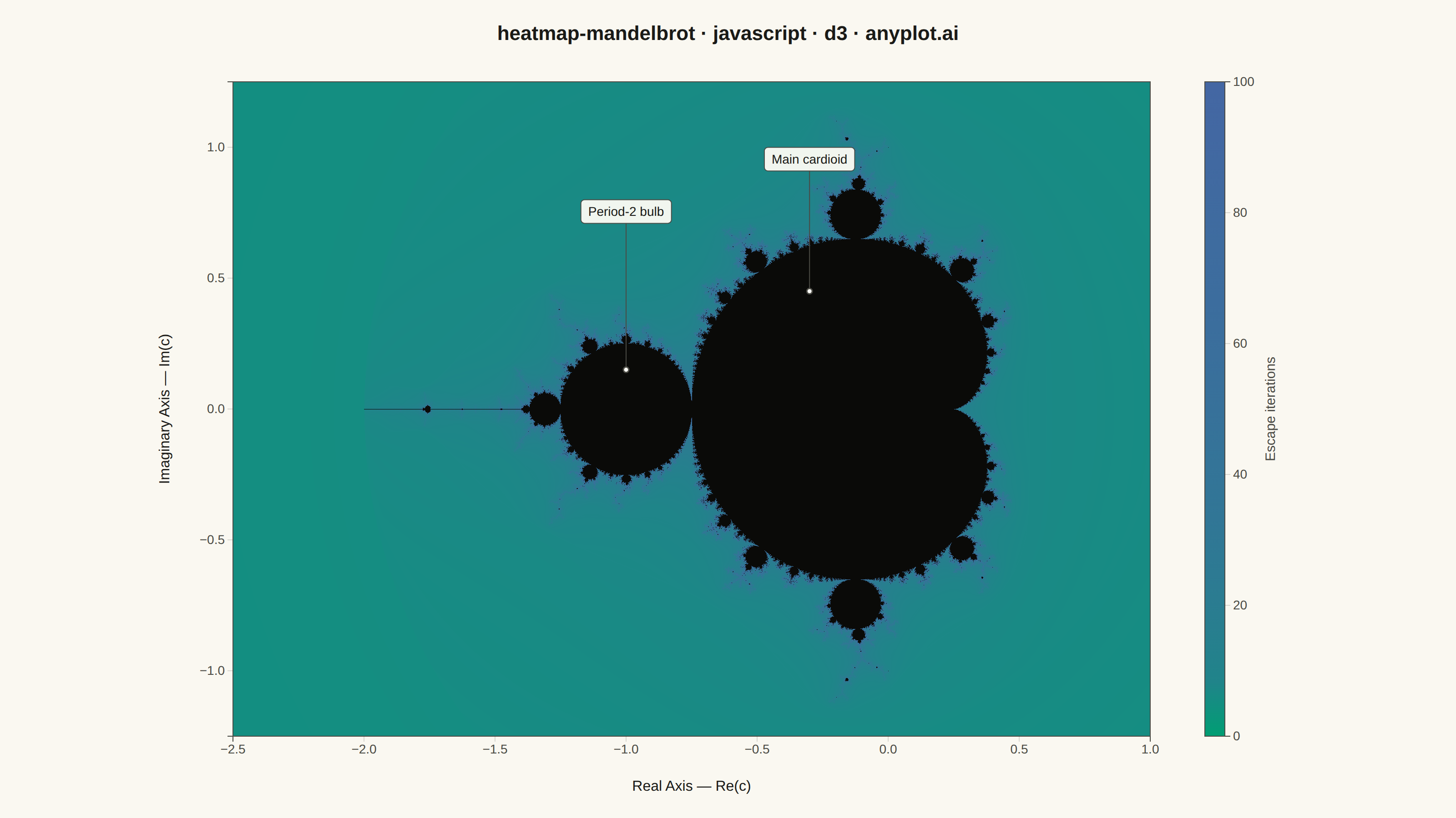
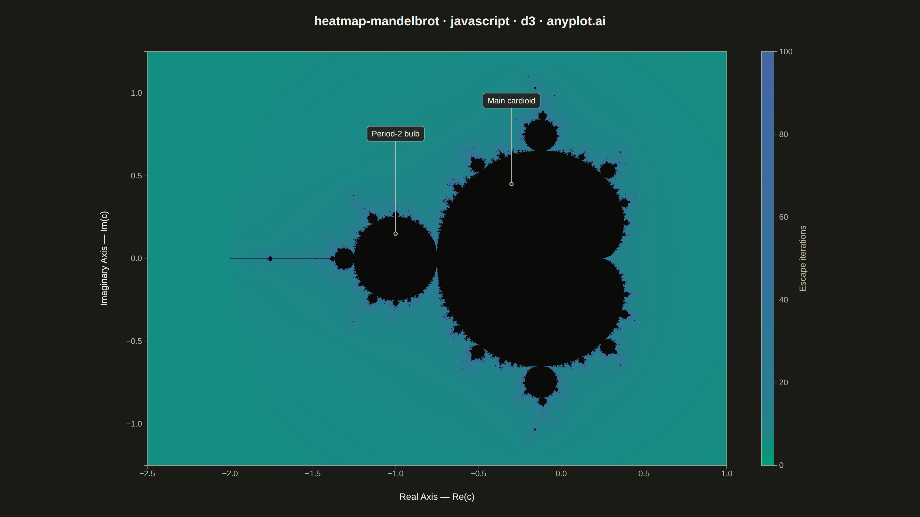
A visualization of the Mandelbrot set, the most iconic fractal in mathematics. Each pixel represents a complex number c on the complex plane, colored by how quickly the iteration z(n+1) = z(n)^2 + c diverges. The boundary between convergent and divergent regions reveals infinitely complex, self-similar structure including the characteristic cardioid and period-2 bulb.
// anyplot.ai
// heatmap-mandelbrot: Mandelbrot Set Fractal Visualization
// Library: d3 7.9.0 | JavaScript 22.23.2
// Quality: 93/100 | Created: 2026-08-25

const tok = window.ANYPLOT_TOKENS;
const { width, height } = window.ANYPLOT_SIZE;

// --- Complex-plane bounds (spec defaults) -----------------------------------
const xMin = -2.5;
const xMax = 1.0;
const yMin = -1.25;
const yMax = 1.25;
const maxIterations = 100;
const bailoutSq = 4; // |z|^2 escape radius^2

// Contrast-curve exponent applied to the normalized escape fraction before it
// hits the LUT. Most background pixels escape within a handful of iterations,
// so a low exponent (well below 1) pushes that dense low-iteration cluster
// further along the green->blue ramp, spreading perceptual detail across the
// escape zone instead of leaving it a flat near-uniform green.
const COLOR_GAMMA = 0.3;

// --- Layout -------------------------------------------------------------------
// Reserve space for title, axis labels/ticks, and a colorbar on the right.
const margin = { top: 90, right: 190, bottom: 90, left: 110 };
const availW = width - margin.left - margin.right;
const availH = height - margin.top - margin.bottom;

// Fit the largest rectangle matching the complex plane's aspect ratio inside
// the available area, then center it — this keeps circles circular instead of
// stretching the fractal to fill the mount.
const dataAspect = (xMax - xMin) / (yMax - yMin);
let plotW = availW;
let plotH = plotW / dataAspect;
if (plotH > availH) {
  plotH = availH;
  plotW = plotH * dataAspect;
}
const plotX = margin.left + (availW - plotW) / 2;
const plotY = margin.top + (availH - plotH) / 2;

// --- Escape-time raster (rendered off-DOM on a <canvas>) --------------------
const DPR = 2; // matches the harness deviceScaleFactor so the raster lands on exact device pixels
const canvasW = Math.round(plotW * DPR);
const canvasH = Math.round(plotH * DPR);
const rasterCanvas = document.createElement("canvas");
rasterCanvas.width = canvasW;
rasterCanvas.height = canvasH;
const ctx = rasterCanvas.getContext("2d");
const imageData = ctx.createImageData(canvasW, canvasH);
const pixels = imageData.data;

// Precompute a 256-step lookup along the Imprint sequential ramp (brand green
// -> blue) so the hot per-pixel loop never allocates or parses a color string.
const seqInterpolator = d3.interpolateRgb(tok.seq[0], tok.seq[1]);
const LUT_STEPS = 256;
const lut = new Uint8Array(LUT_STEPS * 3);
for (let i = 0; i < LUT_STEPS; i++) {
  const c = d3.rgb(seqInterpolator(i / (LUT_STEPS - 1)));
  lut[i * 3] = c.r;
  lut[i * 3 + 1] = c.g;
  lut[i * 3 + 2] = c.b;
}
const insideColor = d3.rgb("#0A0A08"); // points that never escape — distinct solid fill

for (let py = 0; py < canvasH; py++) {
  const ci0 = yMax - (py / canvasH) * (yMax - yMin);
  for (let px = 0; px < canvasW; px++) {
    const cr = xMin + (px / canvasW) * (xMax - xMin);
    const ci = ci0;

    let zr = 0;
    let zi = 0;
    let n = 0;
    let zr2 = 0;
    let zi2 = 0;
    while (zr2 + zi2 <= bailoutSq && n < maxIterations) {
      zi = 2 * zr * zi + ci;
      zr = zr2 - zi2 + cr;
      zr2 = zr * zr;
      zi2 = zi * zi;
      n++;
    }

    const idx = (py * canvasW + px) * 4;
    if (n >= maxIterations) {
      pixels[idx] = insideColor.r;
      pixels[idx + 1] = insideColor.g;
      pixels[idx + 2] = insideColor.b;
    } else {
      // Smooth (renormalized) escape count avoids discrete color banding.
      const logZn = Math.log(zr2 + zi2) / 2;
      const nu = Math.log(logZn / Math.LN2) / Math.LN2;
      const smoothed = n + 1 - nu;
      const t = Math.pow(Math.min(1, Math.max(0, smoothed / maxIterations)), COLOR_GAMMA);
      const lutIdx = Math.round(t * (LUT_STEPS - 1)) * 3;
      pixels[idx] = lut[lutIdx];
      pixels[idx + 1] = lut[lutIdx + 1];
      pixels[idx + 2] = lut[lutIdx + 2];
    }
    pixels[idx + 3] = 255;
  }
}
ctx.putImageData(imageData, 0, 0);
const rasterDataUrl = rasterCanvas.toDataURL("image/png");

// --- SVG mount ----------------------------------------------------------------
const svg = d3.select("#container").append("svg").attr("width", width).attr("height", height);

svg
  .append("image")
  .attr("x", plotX)
  .attr("y", plotY)
  .attr("width", plotW)
  .attr("height", plotH)
  .attr("href", rasterDataUrl);

svg
  .append("rect")
  .attr("x", plotX)
  .attr("y", plotY)
  .attr("width", plotW)
  .attr("height", plotH)
  .attr("fill", "none")
  .attr("stroke", tok.inkSoft)
  .attr("stroke-width", 1);

// --- Axes (real / imaginary parts of c) ---------------------------------------
const x = d3.scaleLinear().domain([xMin, xMax]).range([0, plotW]);
const y = d3.scaleLinear().domain([yMin, yMax]).range([plotH, 0]);

const xAxis = svg
  .append("g")
  .attr("transform", `translate(${plotX},${plotY + plotH})`)
  .call(d3.axisBottom(x).ticks(7));
const yAxis = svg
  .append("g")
  .attr("transform", `translate(${plotX},${plotY})`)
  .call(d3.axisLeft(y).ticks(7));

for (const axisG of [xAxis, yAxis]) {
  axisG.selectAll("text").attr("fill", tok.inkSoft).style("font-size", "14px");
  axisG.selectAll("line").attr("stroke", tok.grid);
  axisG.select(".domain").attr("stroke", tok.inkSoft);
}

svg
  .append("text")
  .attr("x", plotX + plotW / 2)
  .attr("y", plotY + plotH + 60)
  .attr("text-anchor", "middle")
  .attr("fill", tok.ink)
  .style("font-size", "16px")
  .text("Real Axis — Re(c)");

svg
  .append("text")
  .attr("transform", `translate(${plotX - 70},${plotY + plotH / 2}) rotate(-90)`)
  .attr("text-anchor", "middle")
  .attr("fill", tok.ink)
  .style("font-size", "16px")
  .text("Imaginary Axis — Im(c)");

// --- Landmark annotations (data storytelling) ----------------------------
// Callout the two features the spec names explicitly: the main cardioid and
// the period-2 bulb tangent to it at c = -0.75. Labels sit on a pill so they
// stay legible over both the black interior and the green/blue escape field.
function addLandmark(dataX, targetDataY, labelDataY, text) {
  const px = plotX + x(dataX);
  const targetPy = plotY + y(targetDataY);
  const labelPy = plotY + y(labelDataY);

  svg
    .append("line")
    .attr("x1", px)
    .attr("y1", targetPy)
    .attr("x2", px)
    .attr("y2", labelPy)
    .attr("stroke", tok.inkSoft)
    .attr("stroke-width", 1);

  svg
    .append("circle")
    .attr("cx", px)
    .attr("cy", targetPy)
    .attr("r", 3)
    .attr("fill", tok.elevatedBg)
    .attr("stroke", tok.inkSoft)
    .attr("stroke-width", 1.5);

  const labelText = svg
    .append("text")
    .attr("x", px)
    .attr("y", labelPy)
    .attr("text-anchor", "middle")
    .attr("dominant-baseline", "middle")
    .attr("fill", tok.ink)
    .style("font-size", "14px")
    .style("font-weight", "500")
    .text(text);

  const bbox = labelText.node().getBBox();
  const padX = 8;
  const padY = 5;
  svg
    .insert("rect", () => labelText.node())
    .attr("x", bbox.x - padX)
    .attr("y", bbox.y - padY)
    .attr("width", bbox.width + padX * 2)
    .attr("height", bbox.height + padY * 2)
    .attr("rx", 4)
    .attr("fill", tok.elevatedBg)
    .attr("stroke", tok.inkSoft)
    .attr("stroke-width", 1)
    .attr("opacity", 0.94);
}

addLandmark(-0.3, 0.45, 0.95, "Main cardioid");
addLandmark(-1.0, 0.15, 0.75, "Period-2 bulb");

// --- Colorbar legend (escape-iteration scale) ---------------------------------
const legendW = 22;
const legendH = plotH;
const legendX = plotX + plotW + 60;
const legendY = plotY;

const gradientId = "mandelbrot-escape-gradient";
const defs = svg.append("defs");
const gradient = defs
  .append("linearGradient")
  .attr("id", gradientId)
  .attr("x1", "0%")
  .attr("y1", "100%")
  .attr("x2", "0%")
  .attr("y2", "0%");

const GRADIENT_STOPS = 12;
for (let i = 0; i <= GRADIENT_STOPS; i++) {
  const frac = i / GRADIENT_STOPS;
  const t = Math.pow(frac, COLOR_GAMMA); // matches the raster's contrast curve
  gradient
    .append("stop")
    .attr("offset", `${frac * 100}%`)
    .attr("stop-color", seqInterpolator(t));
}

svg
  .append("rect")
  .attr("x", legendX)
  .attr("y", legendY)
  .attr("width", legendW)
  .attr("height", legendH)
  .attr("fill", `url(#${gradientId})`)
  .attr("stroke", tok.inkSoft)
  .attr("stroke-width", 1);

const legendScale = d3.scaleLinear().domain([0, maxIterations]).range([legendH, 0]);
const legendAxis = svg
  .append("g")
  .attr("transform", `translate(${legendX + legendW},${legendY})`)
  .call(d3.axisRight(legendScale).ticks(5));
legendAxis.selectAll("text").attr("fill", tok.inkSoft).style("font-size", "14px");
legendAxis.selectAll("line").attr("stroke", tok.grid);
legendAxis.select(".domain").attr("stroke", tok.inkSoft);

svg
  .append("text")
  .attr("transform", `translate(${legendX + legendW + 55},${legendY + legendH / 2}) rotate(-90)`)
  .attr("text-anchor", "middle")
  .attr("fill", tok.inkSoft)
  .style("font-size", "15px")
  .text("Escape iterations");

// --- Title ----------------------------------------------------------------
svg
  .append("text")
  .attr("x", width / 2)
  .attr("y", 44)
  .attr("text-anchor", "middle")
  .attr("fill", tok.ink)
  .style("font-size", "22px")
  .style("font-weight", "600")
  .text("heatmap-mandelbrot · javascript · d3 · anyplot.ai");
Runnable source as JSON, for any HTTP client: https://api.anyplot.ai/specs/heatmap-mandelbrot/d3/code. Any spec id and library id listed in llms-full.txt fit the same URL shape; every URL below is complete and callable.
{
  "spec_id": "heatmap-mandelbrot",
  "language": "javascript",
  "library": "d3",
  "page": "https://anyplot.ai/heatmap-mandelbrot/javascript/d3",
  "hub": "https://anyplot.ai/heatmap-mandelbrot",
  "code_json": "https://api.anyplot.ai/specs/heatmap-mandelbrot/d3/code",
  "spec_json": "https://api.anyplot.ai/specs/heatmap-mandelbrot",
  "render_light_png": "https://storage.googleapis.com/anyplot-images/plots/heatmap-mandelbrot/javascript/d3/plot-light.png",
  "render_dark_png": "https://storage.googleapis.com/anyplot-images/plots/heatmap-mandelbrot/javascript/d3/plot-dark.png",
  "interactive_light_html": "https://storage.googleapis.com/anyplot-images/plots/heatmap-mandelbrot/javascript/d3/plot-light.html",
  "interactive_dark_html": "https://storage.googleapis.com/anyplot-images/plots/heatmap-mandelbrot/javascript/d3/plot-dark.html",
  "quality_score": 93.0,
  "license": "MIT",
  "guide": "https://anyplot.ai/llms.txt"
}
Part of Mandelbrot Set Fractal Visualization on anyplot.ai.