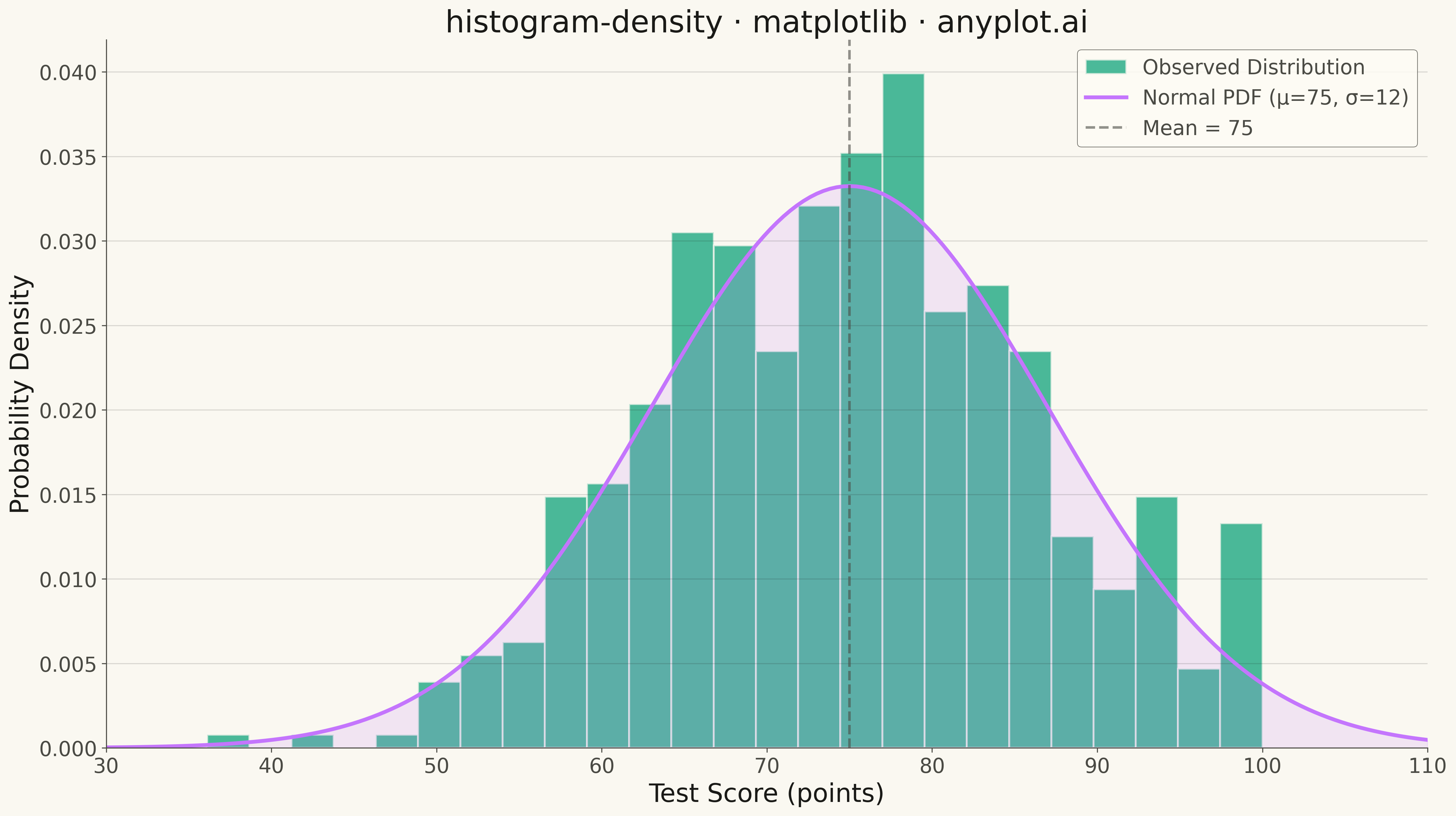
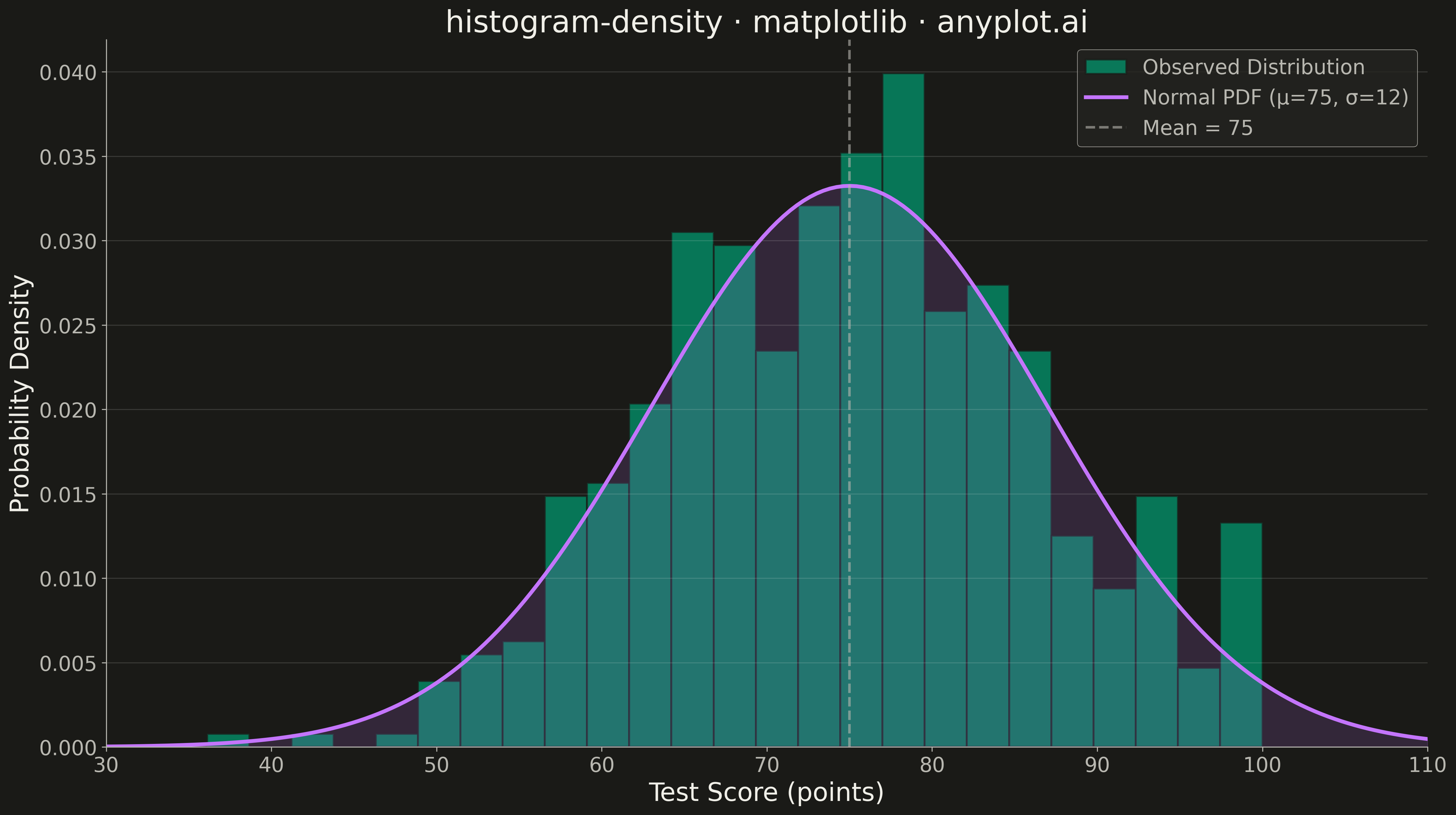
A density histogram displays the distribution of a continuous variable normalized so that the total area under the histogram equals 1, representing probability density instead of raw counts. This normalization allows direct comparison between distributions with different sample sizes and enables overlaying theoretical probability density functions (PDFs) for statistical analysis.
""" anyplot.ai
histogram-density: Density Histogram
Library: matplotlib 3.10.9 | Python 3.13.13
Quality: 89/100 | Updated: 2026-05-11
"""

import os

import matplotlib.pyplot as plt
import numpy as np


# Theme tokens
THEME = os.getenv("ANYPLOT_THEME", "light")
PAGE_BG = "#FAF8F1" if THEME == "light" else "#1A1A17"
ELEVATED_BG = "#FFFDF6" if THEME == "light" else "#242420"
INK = "#1A1A17" if THEME == "light" else "#F0EFE8"
INK_SOFT = "#4A4A44" if THEME == "light" else "#B8B7B0"

# Okabe-Ito palette
BRAND = "#009E73"  # First categorical series
ACCENT = "#C475FD"  # Second color for overlay

# Data: Generate realistic test score data with a normal distribution
np.random.seed(42)
test_scores = np.random.normal(loc=75, scale=12, size=500)
test_scores = np.clip(test_scores, 0, 100)

# Create theoretical normal PDF for overlay
mu, sigma = 75, 12
x_pdf = np.linspace(30, 110, 200)
pdf = (1 / (sigma * np.sqrt(2 * np.pi))) * np.exp(-0.5 * ((x_pdf - mu) / sigma) ** 2)

# Plot
fig, ax = plt.subplots(figsize=(16, 9), facecolor=PAGE_BG)
ax.set_facecolor(PAGE_BG)

# Density histogram with Okabe-Ito brand color
ax.hist(
    test_scores,
    bins=25,
    density=True,
    alpha=0.7,
    color=BRAND,
    edgecolor=PAGE_BG,
    linewidth=1.5,
    label="Observed Distribution",
)

# Overlay theoretical normal PDF with fill_between for visual distinction
ax.plot(x_pdf, pdf, color=ACCENT, linewidth=3, label="Normal PDF (μ=75, σ=12)")
ax.fill_between(x_pdf, pdf, alpha=0.15, color=ACCENT)

# Add mean line for reference
ax.axvline(mu, color=INK_SOFT, linestyle="--", linewidth=2, alpha=0.6, label=f"Mean = {mu}")

# Labels and styling
ax.set_xlabel("Test Score (points)", fontsize=20, color=INK)
ax.set_ylabel("Probability Density", fontsize=20, color=INK)
ax.set_title("histogram-density · matplotlib · anyplot.ai", fontsize=24, fontweight="medium", color=INK)
ax.tick_params(axis="both", labelsize=16, colors=INK_SOFT)

# Theme-adaptive spine and grid styling
for spine in ("left", "bottom"):
    ax.spines[spine].set_color(INK_SOFT)
ax.spines["top"].set_visible(False)
ax.spines["right"].set_visible(False)
ax.yaxis.grid(True, alpha=0.15, linewidth=0.8, color=INK)

# Legend with theme-adaptive styling
leg = ax.legend(fontsize=16, loc="upper right")
if leg:
    leg.get_frame().set_facecolor(ELEVATED_BG)
    leg.get_frame().set_edgecolor(INK_SOFT)
    leg.get_frame().set_linewidth(0.5)
    plt.setp(leg.get_texts(), color=INK_SOFT)

ax.set_xlim(30, 110)
ax.set_ylim(0, None)

plt.tight_layout()
plt.savefig(f"plot-{THEME}.png", dpi=300, bbox_inches="tight", facecolor=PAGE_BG)
Runnable source as JSON, for any HTTP client: https://api.anyplot.ai/specs/histogram-density/matplotlib/code. Any spec id and library id listed in llms-full.txt fit the same URL shape; every URL below is complete and callable.
{
  "spec_id": "histogram-density",
  "language": "python",
  "library": "matplotlib",
  "page": "https://anyplot.ai/histogram-density/python/matplotlib",
  "hub": "https://anyplot.ai/histogram-density",
  "code_json": "https://api.anyplot.ai/specs/histogram-density/matplotlib/code",
  "spec_json": "https://api.anyplot.ai/specs/histogram-density",
  "render_light_png": "https://storage.googleapis.com/anyplot-images/plots/histogram-density/python/matplotlib/plot-light.png",
  "render_dark_png": "https://storage.googleapis.com/anyplot-images/plots/histogram-density/python/matplotlib/plot-dark.png",
  "quality_score": 89.0,
  "license": "MIT",
  "guide": "https://anyplot.ai/llms.txt"
}
Part of Density Histogram on anyplot.ai.