The same plot in 14 other libraries — Python: Altair, Bokeh, lets-plot, Matplotlib, Plotly, plotnine, Pygal, Seaborn; Julia: Makie.jl; JavaScript: Chart.js, D3.js, Apache ECharts, Highcharts, MUI X Charts. Compare all 15 side by side: RSI Technical Indicator Chart in Python, R, Julia and JavaScript.
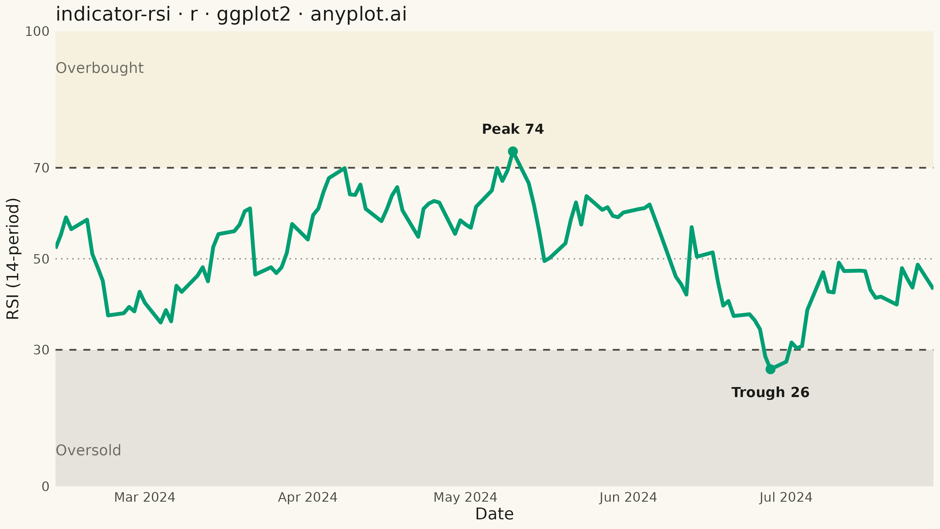
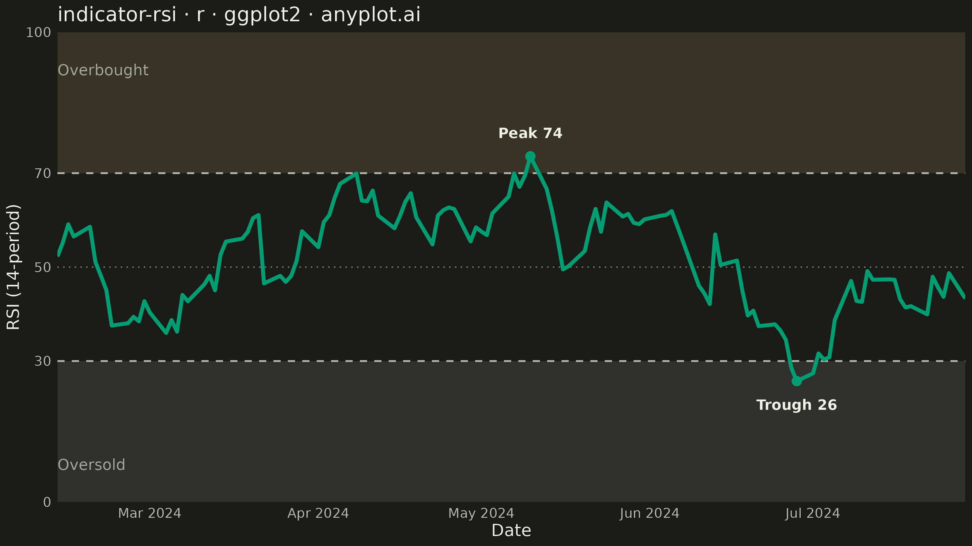
A Relative Strength Index (RSI) chart displaying the momentum oscillator on a 0-100 scale with horizontal threshold lines at 70 (overbought) and 30 (oversold). The RSI measures the speed and magnitude of recent price changes to evaluate overbought or oversold conditions. This is a fundamental momentum indicator in technical analysis, helping traders identify potential reversal points when the market reaches extreme conditions.
#' anyplot.ai
#' indicator-rsi: RSI Technical Indicator Chart
#' Library: ggplot2 3.5.1 | R 4.4.1
#' Quality: 94/100 | Created: 2026-09-05

library(ggplot2)
library(dplyr)
library(ragg)

set.seed(42)

# --- Theme tokens -----------------------------------------------------------
THEME       <- Sys.getenv("ANYPLOT_THEME", "light")
PAGE_BG     <- if (THEME == "light") "#FAF8F1" else "#1A1A17"
INK         <- if (THEME == "light") "#1A1A17" else "#F0EFE8"
INK_SOFT    <- if (THEME == "light") "#4A4A44" else "#B8B7B0"
INK_MUTED   <- if (THEME == "light") "#6B6A63" else "#A8A79F"
ANYPLOT_MUTED <- INK_MUTED

IMPRINT_PALETTE <- c(
  "#009E73", "#C475FD", "#4467A3", "#BD8233",
  "#AE3030", "#2ABCCD", "#954477", "#99B314"
)
BRAND         <- IMPRINT_PALETTE[1] # RSI line — always the brand green
ANYPLOT_AMBER <- "#DDCC77"          # warning anchor — overbought zone

# --- Data: simulate a daily close price series and derive its 14-period RSI -
rsi_period <- 14
calendar_days <- seq(as.Date("2024-01-02"), by = "day", length.out = 210)
trade_dates   <- calendar_days[!weekdays(calendar_days) %in% c("Saturday", "Sunday")]

daily_change <- rnorm(length(trade_dates), mean = 0.15, sd = 2.2)
close_price  <- 150 + cumsum(daily_change)

price_delta <- diff(close_price)
gains  <- pmax(price_delta, 0)
losses <- pmax(-price_delta, 0)

avg_gain <- numeric(length(gains))
avg_loss <- numeric(length(losses))
avg_gain[rsi_period] <- mean(gains[1:rsi_period])
avg_loss[rsi_period] <- mean(losses[1:rsi_period])
for (i in (rsi_period + 1):length(gains)) {
  avg_gain[i] <- (avg_gain[i - 1] * (rsi_period - 1) + gains[i]) / rsi_period
  avg_loss[i] <- (avg_loss[i - 1] * (rsi_period - 1) + losses[i]) / rsi_period
}

relative_strength <- avg_gain / avg_loss
rsi_values <- 100 - (100 / (1 + relative_strength))

df <- tibble::tibble(
  date = trade_dates[(rsi_period + 1):length(trade_dates)],
  rsi  = rsi_values[rsi_period:length(rsi_values)]
) %>%
  filter(!is.na(rsi)) %>%
  slice_tail(n = 120)

# --- Plot ---------------------------------------------------------------
chart_start <- min(df$date)
chart_end   <- max(df$date)

peak_pt   <- df[which.max(df$rsi), ]
trough_pt <- df[which.min(df$rsi), ]

peak_hjust <- ifelse(as.numeric(peak_pt$date - chart_start) < 15, 0,
  ifelse(as.numeric(chart_end - peak_pt$date) < 15, 1, 0.5)
)
trough_hjust <- ifelse(as.numeric(trough_pt$date - chart_start) < 15, 0,
  ifelse(as.numeric(chart_end - trough_pt$date) < 15, 1, 0.5)
)

p <- ggplot(df, aes(date, rsi)) +
  geom_ribbon(aes(ymin = 70, ymax = 100), fill = ANYPLOT_AMBER, alpha = 0.15) +
  geom_ribbon(aes(ymin = 0, ymax = 30), fill = ANYPLOT_MUTED, alpha = 0.15) +
  geom_hline(yintercept = 50, linetype = "dotted", linewidth = 0.4, color = INK_SOFT, alpha = 0.6) +
  geom_hline(yintercept = c(30, 70), linetype = "dashed", linewidth = 0.5, color = INK_SOFT) +
  geom_line(color = BRAND, linewidth = 1.1) +
  annotate("text",
    x = min(df$date), y = 92, label = "Overbought", hjust = 0,
    size = 3.2, color = INK_MUTED
  ) +
  annotate("text",
    x = min(df$date), y = 8, label = "Oversold", hjust = 0,
    size = 3.2, color = INK_MUTED
  ) +
  annotate("point", x = peak_pt$date, y = peak_pt$rsi, color = BRAND, size = 2.2) +
  annotate("text",
    x = peak_pt$date, y = peak_pt$rsi + 5, label = sprintf("Peak %.0f", peak_pt$rsi),
    hjust = peak_hjust, size = 3, color = INK, fontface = "bold"
  ) +
  annotate("point", x = trough_pt$date, y = trough_pt$rsi, color = BRAND, size = 2.2) +
  annotate("text",
    x = trough_pt$date, y = trough_pt$rsi - 5, label = sprintf("Trough %.0f", trough_pt$rsi),
    hjust = trough_hjust, size = 3, color = INK, fontface = "bold"
  ) +
  scale_y_continuous(limits = c(0, 100), breaks = c(0, 30, 50, 70, 100), expand = c(0, 0)) +
  scale_x_date(date_labels = "%b %Y", date_breaks = "1 month", expand = c(0, 0)) +
  labs(
    title = "indicator-rsi · r · ggplot2 · anyplot.ai",
    x = "Date",
    y = "RSI (14-period)"
  ) +
  theme_minimal(base_size = 8) +
  theme(
    text              = element_text(size = 7, color = INK),
    plot.background   = element_rect(fill = PAGE_BG, color = PAGE_BG),
    panel.background  = element_rect(fill = PAGE_BG, color = NA),
    panel.grid.major.x = element_blank(),
    panel.grid.minor   = element_blank(),
    panel.grid.major.y = element_blank(),
    axis.title        = element_text(color = INK, size = 10),
    axis.text         = element_text(color = INK_SOFT, size = 8),
    axis.ticks        = element_blank(),
    plot.title        = element_text(color = INK, size = 12),
    legend.position   = "none"
  )

# --- Save -----------------------------------------------------------------
ggsave(
  filename = sprintf("plot-%s.png", THEME),
  plot     = p,
  device   = ragg::agg_png,
  width    = 8,
  height   = 4.5,
  units    = "in",
  dpi      = 400
)
Runnable source as JSON, for any HTTP client: https://api.anyplot.ai/specs/indicator-rsi/ggplot2/code. Any spec id and library id listed in llms-full.txt fit the same URL shape; every URL below is complete and callable.
{
  "spec_id": "indicator-rsi",
  "language": "r",
  "library": "ggplot2",
  "page": "https://anyplot.ai/indicator-rsi/r/ggplot2",
  "hub": "https://anyplot.ai/indicator-rsi",
  "code_json": "https://api.anyplot.ai/specs/indicator-rsi/ggplot2/code",
  "spec_json": "https://api.anyplot.ai/specs/indicator-rsi",
  "render_light_png": "https://storage.googleapis.com/anyplot-images/plots/indicator-rsi/r/ggplot2/plot-light.png",
  "render_dark_png": "https://storage.googleapis.com/anyplot-images/plots/indicator-rsi/r/ggplot2/plot-dark.png",
  "quality_score": 94.0,
  "license": "MIT",
  "guide": "https://anyplot.ai/llms.txt"
}
Part of RSI Technical Indicator Chart on anyplot.ai.