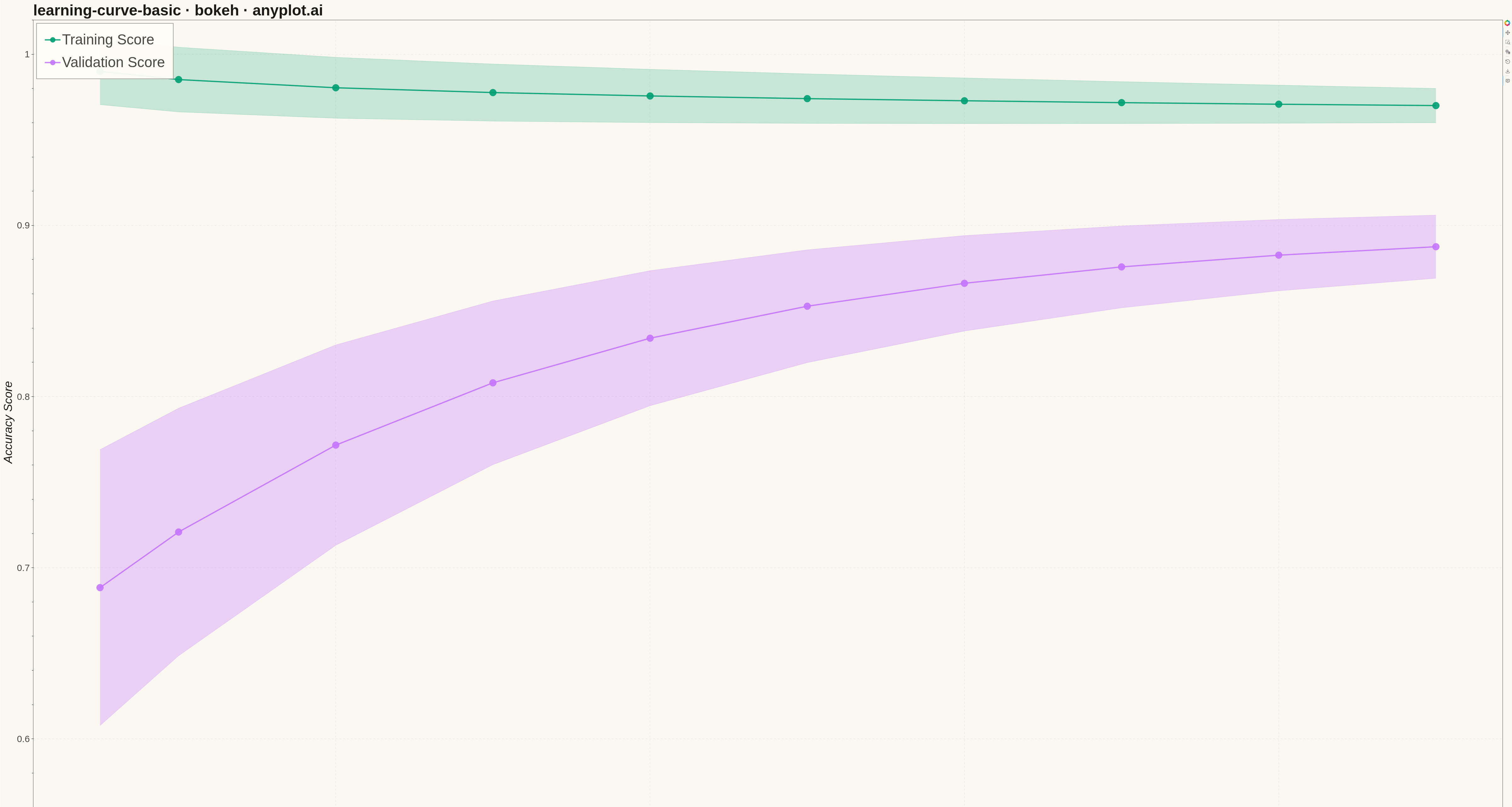
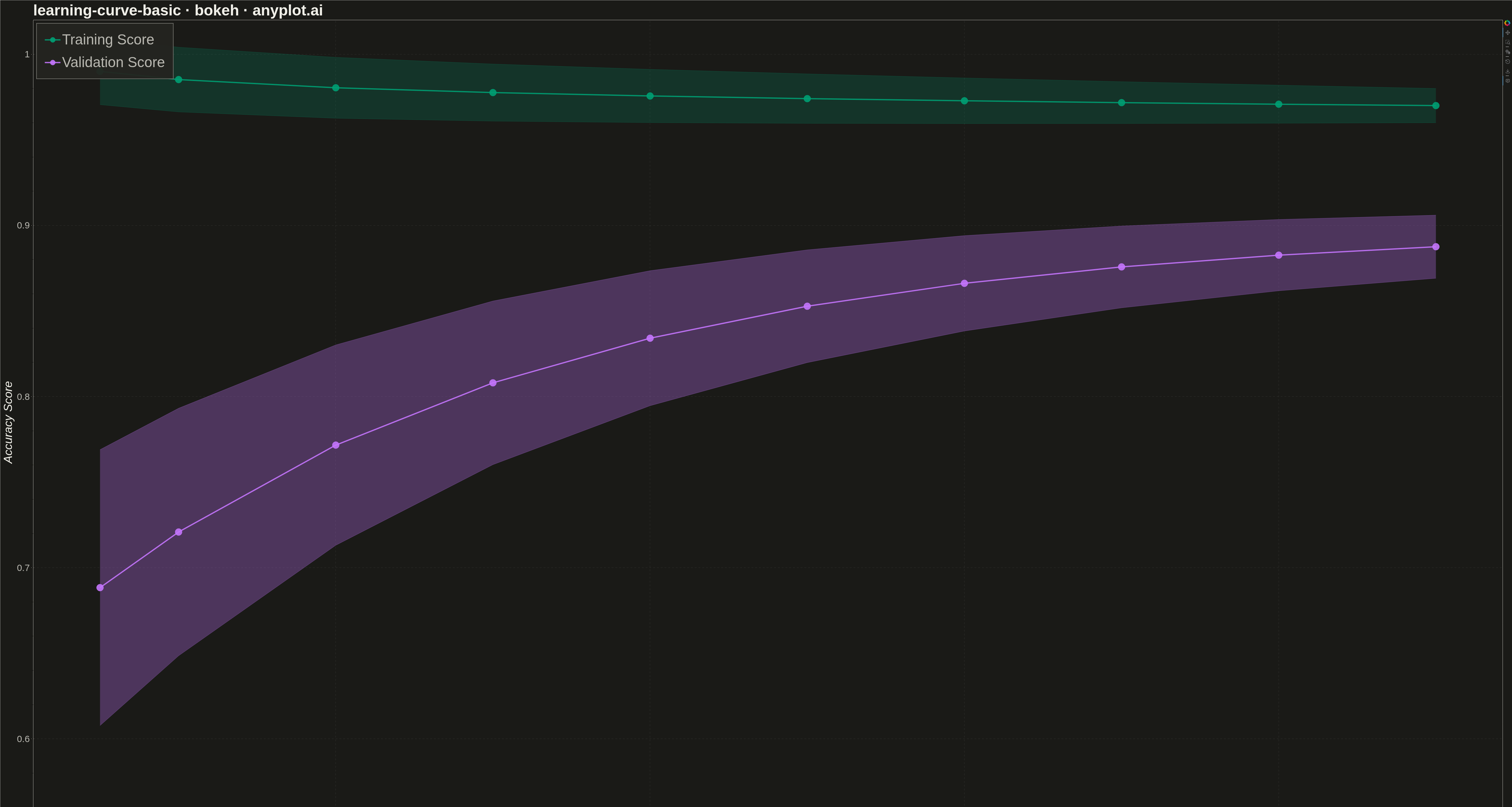
A learning curve visualizes model performance (training and validation scores) as a function of training set size. It is essential for diagnosing bias vs variance tradeoffs, determining whether collecting more data would improve model performance, and guiding model selection decisions. The plot typically shows two lines with shaded confidence bands representing variability across cross-validation folds.
""" anyplot.ai
learning-curve-basic: Model Learning Curve
Library: bokeh 3.9.0 | Python 3.13.13
Quality: 92/100 | Updated: 2026-05-10
"""

import os
import sys
import time
from pathlib import Path


# Remove the script directory from sys.path to avoid importing bokeh.py as bokeh
script_dir = Path(__file__).parent
if str(script_dir) in sys.path:
    sys.path.remove(str(script_dir))

import numpy as np
from bokeh.io import output_file, save
from bokeh.models import Band, ColumnDataSource, HoverTool, Legend, LegendItem
from bokeh.plotting import figure
from selenium import webdriver
from selenium.webdriver.chrome.options import Options


THEME = os.getenv("ANYPLOT_THEME", "light")
PAGE_BG = "#FAF8F1" if THEME == "light" else "#1A1A17"
ELEVATED_BG = "#FFFDF6" if THEME == "light" else "#242420"
INK = "#1A1A17" if THEME == "light" else "#F0EFE8"
INK_SOFT = "#4A4A44" if THEME == "light" else "#B8B7B0"

# Okabe-Ito palette
TRAIN_COLOR = "#009E73"  # Position 1: brand green
VAL_COLOR = "#C475FD"  # Position 2: vermillion

# Data - Simulate learning curve for a classification model
np.random.seed(42)

# Training set sizes (10 points from 10% to 100% of data)
train_sizes = np.array([50, 100, 200, 300, 400, 500, 600, 700, 800, 900])

# Simulate 5-fold cross-validation scores
n_folds = 5
n_sizes = len(train_sizes)

# Training scores: start high and stay high (slight decrease as model generalizes)
train_scores_mean = 0.99 - 0.02 * np.log(train_sizes / train_sizes[0]) / np.log(train_sizes[-1] / train_sizes[0])
train_scores_std = 0.01 + 0.01 * (1 - train_sizes / train_sizes[-1])

# Validation scores: start low, improve with more data (typical learning curve shape)
validation_scores_mean = 0.65 + 0.25 * (1 - np.exp(-train_sizes / 300))
validation_scores_std = 0.08 * np.exp(-train_sizes / 400) + 0.01

# Create bands for confidence intervals (±1 std)
train_upper = train_scores_mean + train_scores_std
train_lower = train_scores_mean - train_scores_std
val_upper = validation_scores_mean + validation_scores_std
val_lower = validation_scores_mean - validation_scores_std

# Create ColumnDataSource for training data
train_source = ColumnDataSource(
    data={"x": train_sizes, "y": train_scores_mean, "upper": train_upper, "lower": train_lower}
)

# Create ColumnDataSource for validation data
val_source = ColumnDataSource(
    data={"x": train_sizes, "y": validation_scores_mean, "upper": val_upper, "lower": val_lower}
)

# Create figure (4800 x 2700 px for 16:9)
p = figure(
    width=4800,
    height=2700,
    title="learning-curve-basic · bokeh · anyplot.ai",
    x_axis_label="Training Set Size (samples)",
    y_axis_label="Accuracy Score",
    tools="pan,wheel_zoom,box_zoom,reset,save",
)

# Add confidence bands for training scores (Okabe-Ito: brand green)
train_band = Band(
    base="x",
    lower="lower",
    upper="upper",
    source=train_source,
    fill_color=TRAIN_COLOR,
    fill_alpha=0.2,
    line_color=TRAIN_COLOR,
    line_alpha=0.3,
)
p.add_layout(train_band)

# Add confidence bands for validation scores (Okabe-Ito: vermillion)
val_band = Band(
    base="x",
    lower="lower",
    upper="upper",
    source=val_source,
    fill_color=VAL_COLOR,
    fill_alpha=0.3,
    line_color=VAL_COLOR,
    line_alpha=0.4,
)
p.add_layout(val_band)

# Plot training score line
train_line = p.line(x="x", y="y", source=train_source, line_color=TRAIN_COLOR, line_width=4, line_alpha=0.9)

# Plot training score markers
train_scatter = p.scatter(x="x", y="y", source=train_source, color=TRAIN_COLOR, size=22, alpha=0.9)

# Plot validation score line
val_line = p.line(x="x", y="y", source=val_source, line_color=VAL_COLOR, line_width=4, line_alpha=0.9)

# Plot validation score markers
val_scatter = p.scatter(x="x", y="y", source=val_source, color=VAL_COLOR, size=22, alpha=0.9)

# Add hover tool for interactivity (Bokeh distinctive feature)
hover_train = HoverTool(
    renderers=[train_scatter],
    tooltips=[
        ("Type", "Training Score"),
        ("Samples", "@x{0}"),
        ("Accuracy", "@y{0.000}"),
        ("Std Range", "@lower{0.000} - @upper{0.000}"),
    ],
    mode="mouse",
)
p.add_tools(hover_train)

hover_val = HoverTool(
    renderers=[val_scatter],
    tooltips=[
        ("Type", "Validation Score"),
        ("Samples", "@x{0}"),
        ("Accuracy", "@y{0.000}"),
        ("Std Range", "@lower{0.000} - @upper{0.000}"),
    ],
    mode="mouse",
)
p.add_tools(hover_val)

# Create legend - positioned inside plot area, top-left for better visibility
legend = Legend(
    items=[
        LegendItem(label="Training Score", renderers=[train_line, train_scatter]),
        LegendItem(label="Validation Score", renderers=[val_line, val_scatter]),
    ],
    location="top_left",
)

p.add_layout(legend, "center")

# Styling - increased sizes for better readability on 4800x2700 canvas
p.title.text_font_size = "36pt"
p.title.text_font_style = "bold"
p.title.text_color = INK
p.xaxis.axis_label_text_font_size = "28pt"
p.yaxis.axis_label_text_font_size = "28pt"
p.xaxis.major_label_text_font_size = "22pt"
p.yaxis.major_label_text_font_size = "22pt"
p.xaxis.axis_label_text_color = INK
p.yaxis.axis_label_text_color = INK
p.xaxis.major_label_text_color = INK_SOFT
p.yaxis.major_label_text_color = INK_SOFT
p.xaxis.axis_line_color = INK_SOFT
p.yaxis.axis_line_color = INK_SOFT
p.xaxis.major_tick_line_color = INK_SOFT
p.yaxis.major_tick_line_color = INK_SOFT

# Legend styling - larger and more prominent
p.legend.label_text_font_size = "34pt"
p.legend.background_fill_alpha = 0.95
p.legend.background_fill_color = ELEVATED_BG
p.legend.border_line_color = INK_SOFT
p.legend.border_line_width = 2
p.legend.label_text_color = INK_SOFT
p.legend.padding = 25
p.legend.spacing = 20
p.legend.glyph_width = 50
p.legend.glyph_height = 40

# Grid styling
p.grid.grid_line_alpha = 0.10
p.grid.grid_line_dash = "dashed"
p.grid.grid_line_color = INK

# Axis range to show all data with padding
p.y_range.start = 0.55
p.y_range.end = 1.02

# Theme-adaptive background and borders
p.background_fill_color = PAGE_BG
p.border_fill_color = PAGE_BG
p.outline_line_color = INK_SOFT

# Save as HTML for interactive version
output_file(f"plot-{THEME}.html")
save(p)

# Screenshot with headless Chrome for PNG (Selenium)
W, H = 4800, 2700
opts = Options()
for arg in (
    "--headless=new",
    "--no-sandbox",
    "--disable-dev-shm-usage",
    "--disable-gpu",
    f"--window-size={W},{H}",
    "--hide-scrollbars",
):
    opts.add_argument(arg)
driver = webdriver.Chrome(options=opts)
driver.set_window_size(W, H)
driver.get(f"file://{Path(f'plot-{THEME}.html').resolve()}")
time.sleep(3)  # let bokeh's JS render the canvas
driver.save_screenshot(f"plot-{THEME}.png")
driver.quit()
Runnable source as JSON, for any HTTP client: https://api.anyplot.ai/specs/learning-curve-basic/bokeh/code. Any spec id and library id listed in llms-full.txt fit the same URL shape; every URL below is complete and callable.
{
  "spec_id": "learning-curve-basic",
  "language": "python",
  "library": "bokeh",
  "page": "https://anyplot.ai/learning-curve-basic/python/bokeh",
  "hub": "https://anyplot.ai/learning-curve-basic",
  "code_json": "https://api.anyplot.ai/specs/learning-curve-basic/bokeh/code",
  "spec_json": "https://api.anyplot.ai/specs/learning-curve-basic",
  "render_light_png": "https://storage.googleapis.com/anyplot-images/plots/learning-curve-basic/python/bokeh/plot-light.png",
  "render_dark_png": "https://storage.googleapis.com/anyplot-images/plots/learning-curve-basic/python/bokeh/plot-dark.png",
  "interactive_light_html": "https://storage.googleapis.com/anyplot-images/plots/learning-curve-basic/python/bokeh/plot-light.html",
  "interactive_dark_html": "https://storage.googleapis.com/anyplot-images/plots/learning-curve-basic/python/bokeh/plot-dark.html",
  "quality_score": 92.0,
  "license": "MIT",
  "guide": "https://anyplot.ai/llms.txt"
}
Part of Model Learning Curve on anyplot.ai.