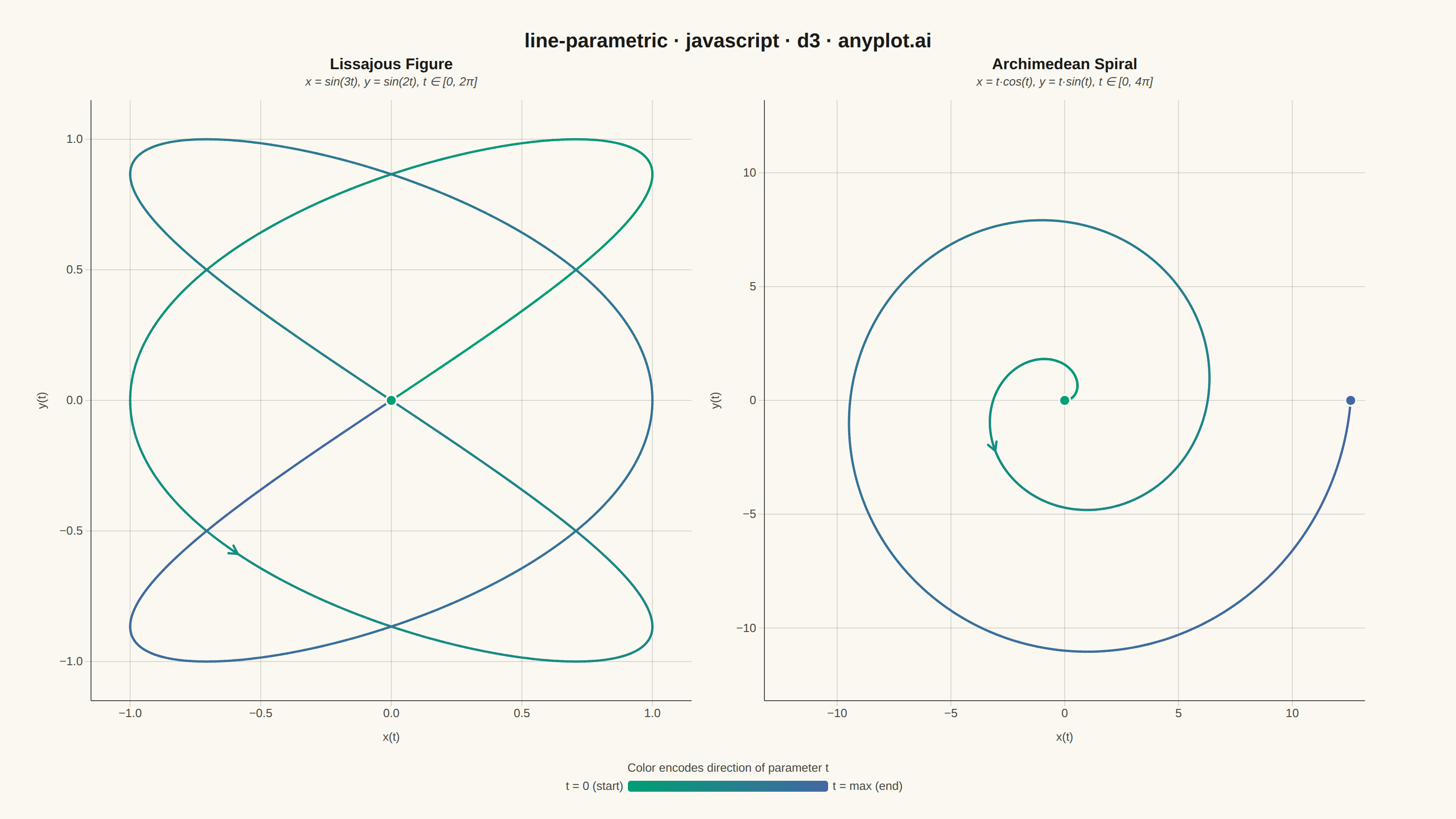
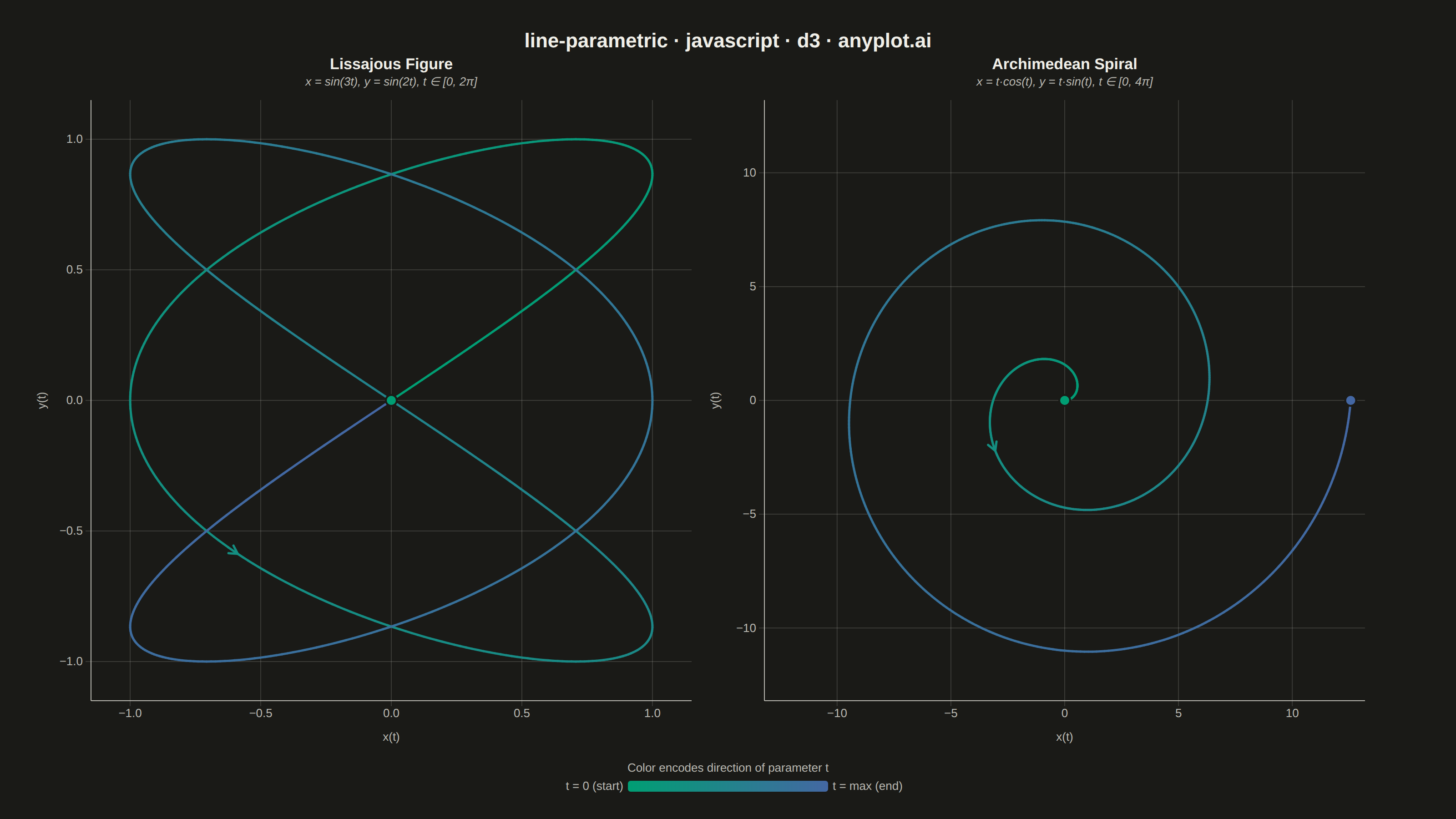
The same plot in 14 other libraries — JavaScript: Chart.js, Apache ECharts, Highcharts, MUI X Charts; Python: Altair, Bokeh, lets-plot, Matplotlib, Plotly, plotnine, Pygal, Seaborn; R: ggplot2; Julia: Makie.jl. Compare all 15 side by side: Parametric Curve Plot in Python, R, Julia and JavaScript.
A parametric curve plot visualizes x(t) and y(t) as functions of a parameter t, tracing smooth curves in 2D space. Unlike standard function plots where y = f(x), parametric curves can loop, self-intersect, and form closed shapes such as Lissajous figures, spirals, and cardioids. This makes them essential for representing trajectories, oscillations, and classical mathematical curves that cannot be expressed as single-valued functions.
// anyplot.ai
// line-parametric: Parametric Curve Plot
// Library: d3 7.9.0 | JavaScript 22.22.3
// Quality: 88/100 | Created: 2026-06-20

const tok = window.ANYPLOT_TOKENS;
const { width, height } = window.ANYPLOT_SIZE;

// Sequential Imprint colormap: green (t=0) → blue (t=max)
const colorT = d3.interpolateRgbBasis(tok.seq);

// --- Data (in-memory, deterministic) ---
const N = 800;
const TWO_PI = 2 * Math.PI;

// Lissajous figure: x = sin(3t), y = sin(2t), t ∈ [0, 2π]
const lissajous = Array.from({ length: N + 1 }, (_, i) => {
  const p = (i / N) * TWO_PI;
  return { u: i / N, x: Math.sin(3 * p), y: Math.sin(2 * p) };
});

// Archimedean spiral: x = t·cos(t), y = t·sin(t), t ∈ [0, 4π]
const T_SPIRAL = 4 * Math.PI;
const spiral = Array.from({ length: N + 1 }, (_, i) => {
  const p = (i / N) * T_SPIRAL;
  return { u: i / N, x: p * Math.cos(p), y: p * Math.sin(p) };
});

// --- SVG mount ---
const svg = d3.select("#container").append("svg")
  .attr("width", width).attr("height", height);

// Gradient definition for the legend bar
const defs = svg.append("defs");
const gradDef = defs.append("linearGradient").attr("id", "tSeq")
  .attr("x1", "0%").attr("x2", "100%");
for (let i = 0; i <= 10; i++) {
  gradDef.append("stop").attr("offset", `${i * 10}%`).attr("stop-color", colorT(i / 10));
}

// --- Layout: two square panels side by side ---
const panelSize = 660;
const panelGap = 80;
const startX = Math.floor((width - (2 * panelSize + panelGap)) / 2);
const startY = 110;

// --- Helper: render one panel ---
function drawPanel(points, xDomain, yDomain, titleText, formulaText, px, py) {
  const xSc = d3.scaleLinear().domain(xDomain).range([0, panelSize]);
  const ySc = d3.scaleLinear().domain(yDomain).range([panelSize, 0]);

  const g = svg.append("g").attr("transform", `translate(${px},${py})`);

  // Subtle gridlines (both axes — symmetric plot)
  for (const v of xSc.ticks(5)) {
    g.append("line")
      .attr("x1", xSc(v)).attr("x2", xSc(v)).attr("y1", 0).attr("y2", panelSize)
      .attr("stroke", tok.grid).attr("stroke-width", 1);
  }
  for (const v of ySc.ticks(5)) {
    g.append("line")
      .attr("x1", 0).attr("x2", panelSize).attr("y1", ySc(v)).attr("y2", ySc(v))
      .attr("stroke", tok.grid).attr("stroke-width", 1);
  }

  // Axes
  const xAx = g.append("g").attr("transform", `translate(0,${panelSize})`)
    .call(d3.axisBottom(xSc).ticks(5).tickSizeOuter(0));
  const yAx = g.append("g")
    .call(d3.axisLeft(ySc).ticks(5).tickSizeOuter(0));
  for (const ax of [xAx, yAx]) {
    ax.selectAll("text").attr("fill", tok.inkSoft).style("font-size", "13px");
    ax.selectAll(".tick line").attr("stroke", tok.grid);
    ax.select(".domain").attr("stroke", tok.inkSoft);
  }

  // Curve: colored path segments encoding t-progress (Imprint sequential)
  g.append("g").selectAll("path")
    .data(d3.pairs(points))
    .join("path")
    .attr("d", ([a, b]) => `M${xSc(a.x)},${ySc(a.y)}L${xSc(b.x)},${ySc(b.y)}`)
    .attr("stroke", ([a]) => colorT(a.u))
    .attr("stroke-width", 2.5)
    .attr("stroke-linecap", "round")
    .attr("fill", "none");

  // Direction chevron at ~30% of traversal
  const ai = Math.floor(N * 0.3);
  const pa = points[ai], pb = points[ai + 1];
  const dx = xSc(pb.x) - xSc(pa.x);
  const dy = ySc(pb.y) - ySc(pa.y);
  const ang = Math.atan2(dy, dx) * 180 / Math.PI;
  g.append("path")
    .attr("d", "M-9,-5 L0,0 L-9,5")
    .attr("transform", `translate(${xSc(pa.x)},${ySc(pa.y)}) rotate(${ang})`)
    .attr("stroke", colorT(0.3))
    .attr("stroke-width", 2.5)
    .attr("fill", "none")
    .attr("stroke-linecap", "round")
    .attr("stroke-linejoin", "round");

  // Start dot
  const sp = points[0];
  g.append("circle")
    .attr("cx", xSc(sp.x)).attr("cy", ySc(sp.y))
    .attr("r", 6).attr("fill", colorT(0))
    .attr("stroke", tok.pageBg).attr("stroke-width", 2);

  // End dot (only if distinct from start — Lissajous is a closed curve)
  const ep = points[N];
  const distSE = Math.hypot(xSc(sp.x) - xSc(ep.x), ySc(sp.y) - ySc(ep.y));
  if (distSE > 8) {
    g.append("circle")
      .attr("cx", xSc(ep.x)).attr("cy", ySc(ep.y))
      .attr("r", 6).attr("fill", colorT(1))
      .attr("stroke", tok.pageBg).attr("stroke-width", 2);
  }

  // Panel title
  g.append("text")
    .attr("x", panelSize / 2).attr("y", -34)
    .attr("text-anchor", "middle").attr("fill", tok.ink)
    .style("font-size", "17px").style("font-weight", "600")
    .text(titleText);

  // Formula subtitle (italic for visual hierarchy below panel title)
  g.append("text")
    .attr("x", panelSize / 2).attr("y", -16)
    .attr("text-anchor", "middle").attr("fill", tok.inkSoft)
    .style("font-size", "13px").style("font-style", "italic")
    .text(formulaText);

  // Axis labels
  g.append("text")
    .attr("x", panelSize / 2).attr("y", panelSize + 44)
    .attr("text-anchor", "middle").attr("fill", tok.inkSoft)
    .style("font-size", "13px").text("x(t)");

  g.append("text")
    .attr("transform", `rotate(-90) translate(${-panelSize / 2},${-50})`)
    .attr("text-anchor", "middle").attr("fill", tok.inkSoft)
    .style("font-size", "13px").text("y(t)");
}

// --- Draw panels ---
drawPanel(
  lissajous,
  [-1.15, 1.15], [-1.15, 1.15],
  "Lissajous Figure",
  "x = sin(3t),  y = sin(2t),  t ∈ [0, 2π]",
  startX, startY
);

const maxR = T_SPIRAL * 1.05;
drawPanel(
  spiral,
  [-maxR, maxR], [-maxR, maxR],
  "Archimedean Spiral",
  "x = t·cos(t),  y = t·sin(t),  t ∈ [0, 4π]",
  startX + panelSize + panelGap, startY
);

// --- Direction legend ---
const legendW = 220, legendH = 12;
const legendX = (width - legendW) / 2;
const legendY = height - 42;

svg.append("text")
  .attr("x", width / 2).attr("y", legendY - 10)
  .attr("text-anchor", "middle").attr("fill", tok.inkSoft)
  .style("font-size", "13px")
  .text("Color encodes direction of parameter t");

svg.append("rect")
  .attr("x", legendX).attr("y", legendY)
  .attr("width", legendW).attr("height", legendH)
  .attr("rx", 3).attr("fill", "url(#tSeq)");

svg.append("text")
  .attr("x", legendX - 5).attr("y", legendY + 10)
  .attr("text-anchor", "end").attr("fill", tok.inkSoft).style("font-size", "13px")
  .text("t = 0 (start)");

svg.append("text")
  .attr("x", legendX + legendW + 5).attr("y", legendY + 10)
  .attr("text-anchor", "start").attr("fill", tok.inkSoft).style("font-size", "13px")
  .text("t = max (end)");

// --- Main title ---
svg.append("text")
  .attr("x", width / 2).attr("y", 52)
  .attr("text-anchor", "middle").attr("fill", tok.ink)
  .style("font-size", "22px").style("font-weight", "600")
  .text("line-parametric · javascript · d3 · anyplot.ai");
Runnable source as JSON, for any HTTP client: https://api.anyplot.ai/specs/line-parametric/d3/code. Any spec id and library id listed in llms-full.txt fit the same URL shape; every URL below is complete and callable.
{
  "spec_id": "line-parametric",
  "language": "javascript",
  "library": "d3",
  "page": "https://anyplot.ai/line-parametric/javascript/d3",
  "hub": "https://anyplot.ai/line-parametric",
  "code_json": "https://api.anyplot.ai/specs/line-parametric/d3/code",
  "spec_json": "https://api.anyplot.ai/specs/line-parametric",
  "render_light_png": "https://storage.googleapis.com/anyplot-images/plots/line-parametric/javascript/d3/plot-light.png",
  "render_dark_png": "https://storage.googleapis.com/anyplot-images/plots/line-parametric/javascript/d3/plot-dark.png",
  "interactive_light_html": "https://storage.googleapis.com/anyplot-images/plots/line-parametric/javascript/d3/plot-light.html",
  "interactive_dark_html": "https://storage.googleapis.com/anyplot-images/plots/line-parametric/javascript/d3/plot-dark.html",
  "quality_score": 88.0,
  "license": "MIT",
  "guide": "https://anyplot.ai/llms.txt"
}
Part of Parametric Curve Plot on anyplot.ai.