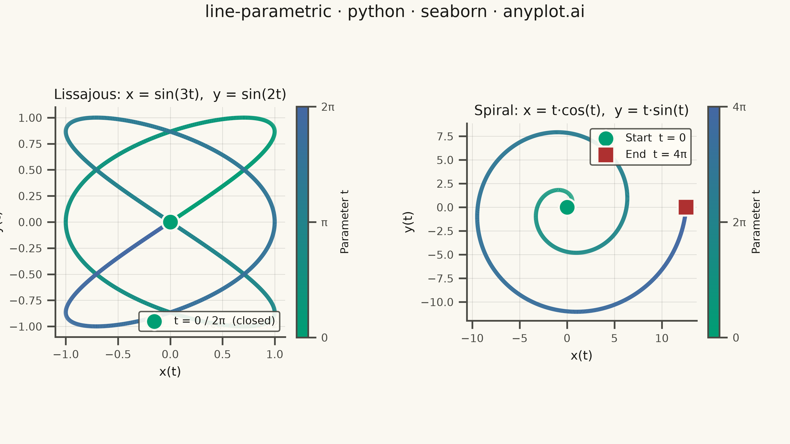
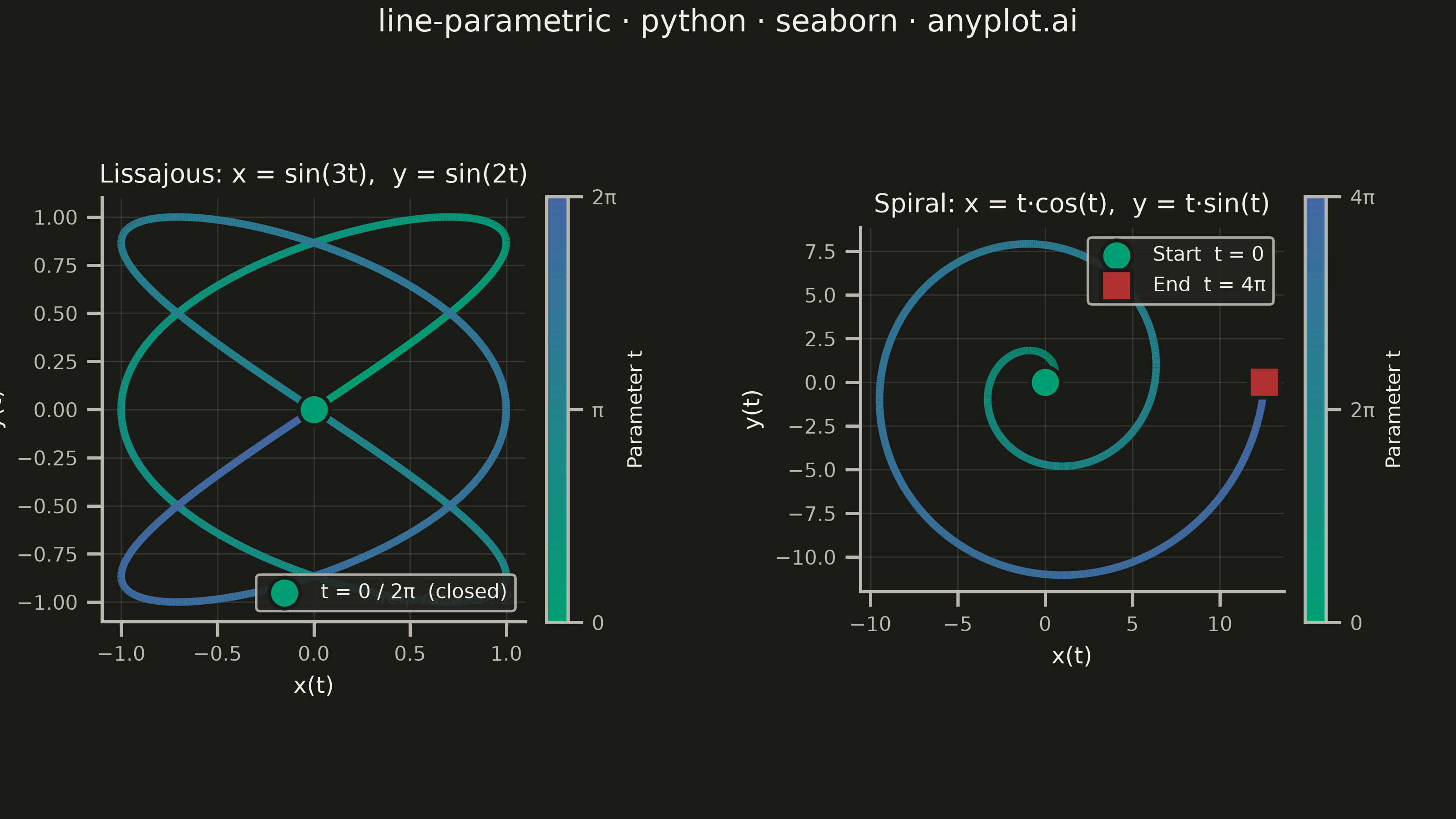
A parametric curve plot visualizes x(t) and y(t) as functions of a parameter t, tracing smooth curves in 2D space. Unlike standard function plots where y = f(x), parametric curves can loop, self-intersect, and form closed shapes such as Lissajous figures, spirals, and cardioids. This makes them essential for representing trajectories, oscillations, and classical mathematical curves that cannot be expressed as single-valued functions.
""" anyplot.ai
line-parametric: Parametric Curve Plot
Library: seaborn 0.13.2 | Python 3.13.14
Quality: 86/100 | Updated: 2026-06-20
"""

import os

import matplotlib.pyplot as plt
import numpy as np
import seaborn as sns
from matplotlib.collections import LineCollection
from matplotlib.colors import LinearSegmentedColormap
from matplotlib.gridspec import GridSpec


# Theme tokens
THEME = os.getenv("ANYPLOT_THEME", "light")
PAGE_BG = "#FAF8F1" if THEME == "light" else "#1A1A17"
ELEVATED_BG = "#FFFDF6" if THEME == "light" else "#242420"
INK = "#1A1A17" if THEME == "light" else "#F0EFE8"
INK_SOFT = "#4A4A44" if THEME == "light" else "#B8B7B0"
INK_MUTED = "#6B6A63" if THEME == "light" else "#A8A79F"

# Imprint sequential colormap: brand green → blue
imprint_seq = LinearSegmentedColormap.from_list("imprint_seq", ["#009E73", "#4467A3"])

# Seaborn theme: warm background + theme-adaptive chrome
sns.set_theme(
    style="ticks",
    rc={
        "figure.facecolor": PAGE_BG,
        "axes.facecolor": PAGE_BG,
        "axes.edgecolor": INK_SOFT,
        "axes.labelcolor": INK,
        "text.color": INK,
        "xtick.color": INK_SOFT,
        "ytick.color": INK_SOFT,
        "grid.color": INK,
        "grid.alpha": 0.12,
        "legend.facecolor": ELEVATED_BG,
        "legend.edgecolor": INK_SOFT,
    },
)

# Data — Lissajous: x = sin(3t), y = sin(2t), t ∈ [0, 2π]
t_liss = np.linspace(0, 2 * np.pi, 1000)
x_liss = np.sin(3 * t_liss)
y_liss = np.sin(2 * t_liss)

# Data — Archimedean spiral: x = t·cos(t), y = t·sin(t), t ∈ [0, 4π]
t_spiral = np.linspace(0, 4 * np.pi, 1000)
x_spiral = t_spiral * np.cos(t_spiral)
y_spiral = t_spiral * np.sin(t_spiral)

# Canvas: 3200 × 1800 px (landscape 16:9)
fig = plt.figure(figsize=(8, 4.5), dpi=400, facecolor=PAGE_BG)
gs = GridSpec(1, 2, figure=fig)
ax1 = fig.add_subplot(gs[0, 0])
ax2 = fig.add_subplot(gs[0, 1])
ax1.set_facecolor(PAGE_BG)
ax2.set_facecolor(PAGE_BG)

# Lissajous — gradient line via inline LineCollection (Imprint sequential cmap)
pts_l = np.column_stack([x_liss, y_liss]).reshape(-1, 1, 2)
segs_l = np.concatenate([pts_l[:-1], pts_l[1:]], axis=1)
lc1 = LineCollection(segs_l, cmap=imprint_seq, linewidths=3)
lc1.set_array(t_liss[:-1])
lc1.set_clim(0, 2 * np.pi)
ax1.add_collection(lc1)
ax1.autoscale()

# Spiral — gradient line via inline LineCollection (Imprint sequential cmap)
pts_s = np.column_stack([x_spiral, y_spiral]).reshape(-1, 1, 2)
segs_s = np.concatenate([pts_s[:-1], pts_s[1:]], axis=1)
lc2 = LineCollection(segs_s, cmap=imprint_seq, linewidths=3)
lc2.set_array(t_spiral[:-1])
lc2.set_clim(0, 4 * np.pi)
ax2.add_collection(lc2)
ax2.autoscale()

# Lissajous is a closed curve (start = end = origin) — single marker
sns.scatterplot(
    x=[x_liss[0]],
    y=[y_liss[0]],
    s=150,
    color="#009E73",
    marker="o",
    zorder=5,
    label="t = 0 / 2π  (closed)",
    edgecolor=PAGE_BG,
    linewidth=1.5,
    ax=ax1,
)

# Spiral: distinct start (green) and end (red) markers
sns.scatterplot(
    x=[x_spiral[0]],
    y=[y_spiral[0]],
    s=150,
    color="#009E73",
    marker="o",
    zorder=5,
    label="Start  t = 0",
    edgecolor=PAGE_BG,
    linewidth=1.5,
    ax=ax2,
)
sns.scatterplot(
    x=[x_spiral[-1]],
    y=[y_spiral[-1]],
    s=150,
    color="#AE3030",
    marker="s",
    zorder=5,
    label="End  t = 4π",
    edgecolor=PAGE_BG,
    linewidth=1.5,
    ax=ax2,
)

# Colorbars with π-symbol tick labels
cb1 = fig.colorbar(lc1, ax=ax1, shrink=0.65, pad=0.04)
cb1.set_label("Parameter t", fontsize=8, color=INK)
cb1.set_ticks([0, np.pi, 2 * np.pi])
cb1.set_ticklabels(["0", "π", "2π"])
cb1.ax.tick_params(labelsize=8, colors=INK_SOFT)

cb2 = fig.colorbar(lc2, ax=ax2, shrink=0.65, pad=0.04)
cb2.set_label("Parameter t", fontsize=8, color=INK)
cb2.set_ticks([0, 2 * np.pi, 4 * np.pi])
cb2.set_ticklabels(["0", "2π", "4π"])
cb2.ax.tick_params(labelsize=8, colors=INK_SOFT)

# Panel styling via seaborn's despine + explicit chrome
for ax, panel_title, legend_loc in [
    (ax1, "Lissajous: x = sin(3t),  y = sin(2t)", "lower right"),
    (ax2, "Spiral: x = t·cos(t),  y = t·sin(t)", "best"),
]:
    ax.set_aspect("equal")
    ax.set_title(panel_title, fontsize=10, fontweight="medium", color=INK)
    ax.set_xlabel("x(t)", fontsize=9, color=INK)
    ax.set_ylabel("y(t)", fontsize=9, color=INK)
    ax.tick_params(axis="both", labelsize=8, colors=INK_SOFT)
    ax.legend(fontsize=8, loc=legend_loc, framealpha=0.9, facecolor=ELEVATED_BG, edgecolor=INK_SOFT)
    ax.grid(True, alpha=0.12, linewidth=0.5, color=INK)
    sns.despine(ax=ax)

# Frequency ratio annotation — data storytelling for Lissajous
ax1.text(
    0.97,
    0.03,
    "freq. ratio  3 : 2",
    transform=ax1.transAxes,
    fontsize=7,
    color=INK_MUTED,
    ha="right",
    va="bottom",
    style="italic",
)

fig.suptitle("line-parametric · python · seaborn · anyplot.ai", fontsize=12, fontweight="medium", color=INK, y=0.99)
fig.subplots_adjust(left=0.07, right=0.95, top=0.90, bottom=0.10, wspace=0.45)

# Save — exact 3200 × 1800 px; no bbox_inches="tight" (would trim canvas)
plt.savefig(f"plot-{THEME}.png", dpi=400, facecolor=PAGE_BG)
Runnable source as JSON, for any HTTP client: https://api.anyplot.ai/specs/line-parametric/seaborn/code. Any spec id and library id listed in llms-full.txt fit the same URL shape; every URL below is complete and callable.
{
  "spec_id": "line-parametric",
  "language": "python",
  "library": "seaborn",
  "page": "https://anyplot.ai/line-parametric/python/seaborn",
  "hub": "https://anyplot.ai/line-parametric",
  "code_json": "https://api.anyplot.ai/specs/line-parametric/seaborn/code",
  "spec_json": "https://api.anyplot.ai/specs/line-parametric",
  "render_light_png": "https://storage.googleapis.com/anyplot-images/plots/line-parametric/python/seaborn/plot-light.png",
  "render_dark_png": "https://storage.googleapis.com/anyplot-images/plots/line-parametric/python/seaborn/plot-dark.png",
  "quality_score": 86.0,
  "license": "MIT",
  "guide": "https://anyplot.ai/llms.txt"
}
Part of Parametric Curve Plot on anyplot.ai.