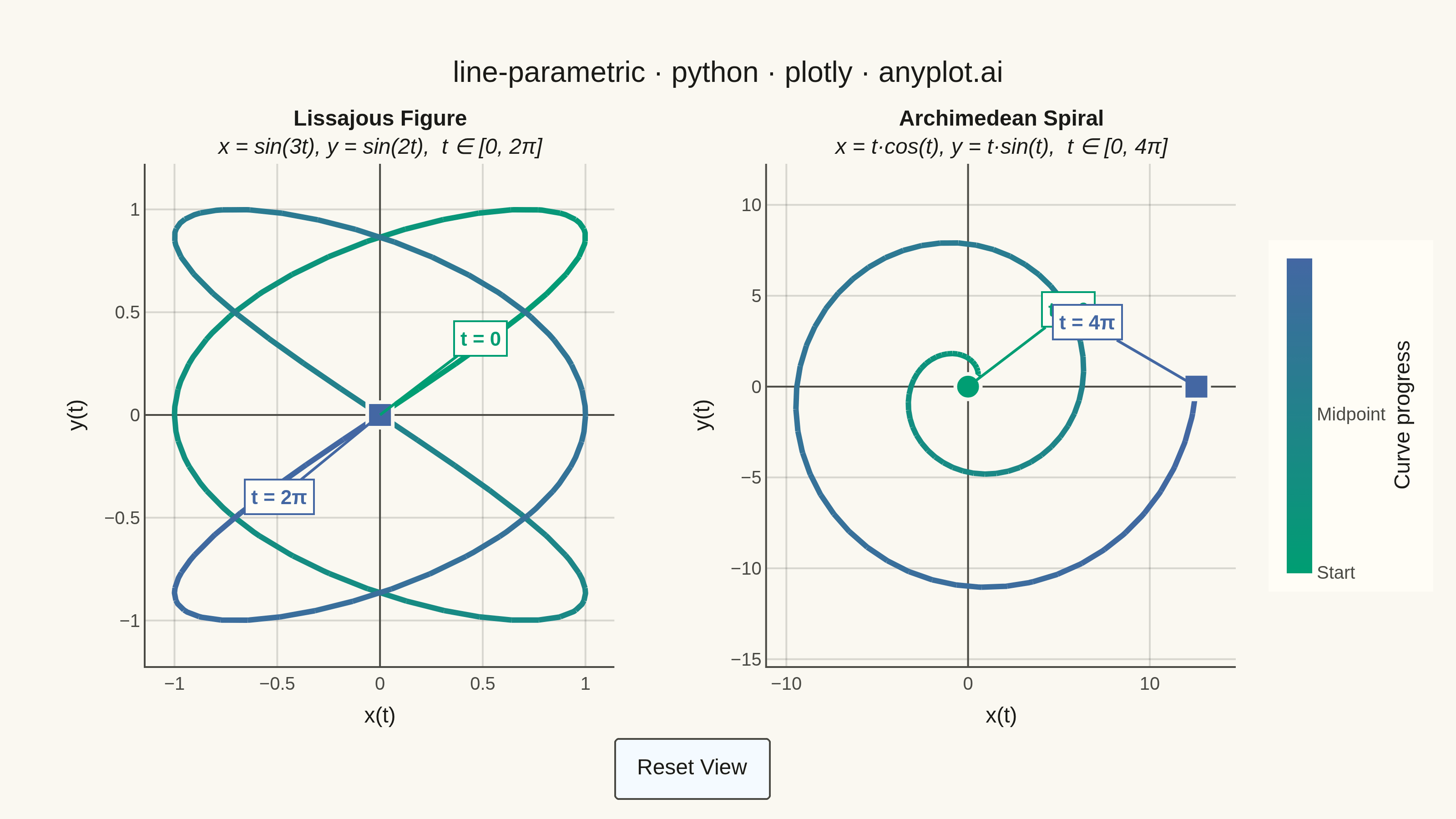
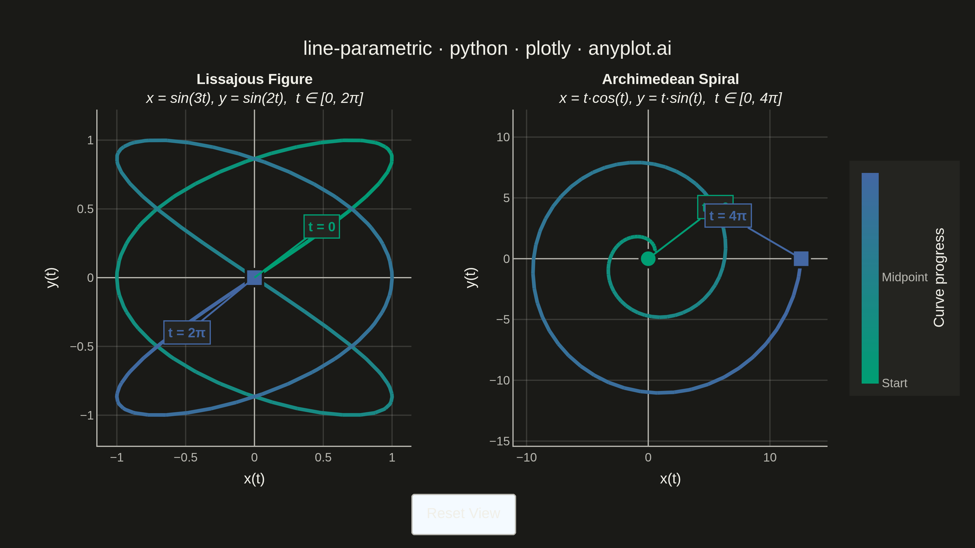
A parametric curve plot visualizes x(t) and y(t) as functions of a parameter t, tracing smooth curves in 2D space. Unlike standard function plots where y = f(x), parametric curves can loop, self-intersect, and form closed shapes such as Lissajous figures, spirals, and cardioids. This makes them essential for representing trajectories, oscillations, and classical mathematical curves that cannot be expressed as single-valued functions.
""" anyplot.ai
line-parametric: Parametric Curve Plot
Library: plotly 6.8.0 | Python 3.13.14
Quality: 90/100 | Updated: 2026-06-20
"""

import os

import numpy as np
import plotly.graph_objects as go
from plotly.subplots import make_subplots


THEME = os.getenv("ANYPLOT_THEME", "light")
PAGE_BG = "#FAF8F1" if THEME == "light" else "#1A1A17"
ELEVATED_BG = "#FFFDF6" if THEME == "light" else "#242420"
INK = "#1A1A17" if THEME == "light" else "#F0EFE8"
INK_SOFT = "#4A4A44" if THEME == "light" else "#B8B7B0"
GRID = "rgba(26,26,23,0.15)" if THEME == "light" else "rgba(240,239,232,0.15)"

# Imprint sequential colorscale: brand green → blue (single-polarity continuous t)
imprint_seq = [[0.0, "#009E73"], [1.0, "#4467A3"]]

# Pre-compute 100 segment colors from Imprint seq palette via numpy (no helper function)
n_seg = 100
c0, c1 = np.array([0x00, 0x9E, 0x73]), np.array([0x44, 0x67, 0xA3])
seg_rgb = (c0 + np.linspace(0, 1, n_seg)[:, None] * (c1 - c0)).astype(int)
seg_colors = [f"rgb({r},{g},{b})" for r, g, b in seg_rgb]

# Data
n_pts = 2000
t_liss = np.linspace(0, 2 * np.pi, n_pts)
x_liss, y_liss = np.sin(3 * t_liss), np.sin(2 * t_liss)

t_spiral = np.linspace(0, 4 * np.pi, n_pts)
x_spiral = t_spiral * np.cos(t_spiral)
y_spiral = t_spiral * np.sin(t_spiral)

# Figure with two subplots
fig = make_subplots(
    rows=1,
    cols=2,
    subplot_titles=(
        "<b>Lissajous Figure</b><br><i>x = sin(3t), y = sin(2t),  t ∈ [0, 2π]</i>",
        "<b>Archimedean Spiral</b><br><i>x = t·cos(t), y = t·sin(t),  t ∈ [0, 4π]</i>",
    ),
    horizontal_spacing=0.14,
)

# Capture subplot title annotation count before adding data annotations
n_title_anns = len(fig.layout.annotations)

seg_size = n_pts // n_seg

for xx, yy, tt, t_max, col_idx, xref, yref, t_end_lbl in [
    (x_liss, y_liss, t_liss, 2 * np.pi, 1, "x", "y", "2π"),
    (x_spiral, y_spiral, t_spiral, 4 * np.pi, 2, "x2", "y2", "4π"),
]:
    # Gradient line segments using pre-computed Imprint palette colors
    for i, color in enumerate(seg_colors):
        s = i * seg_size
        e = min(s + seg_size + 1, n_pts)
        fig.add_trace(
            go.Scatter(
                x=xx[s:e], y=yy[s:e], mode="lines", line=dict(width=3, color=color), showlegend=False, hoverinfo="skip"
            ),
            row=1,
            col=col_idx,
        )

    # Invisible markers for hover + single shared colorbar on far right
    fig.add_trace(
        go.Scatter(
            x=xx[::10],
            y=yy[::10],
            mode="markers",
            marker=dict(
                size=0.1,
                opacity=0,
                color=tt[::10] / t_max,
                colorscale=imprint_seq,
                showscale=(col_idx == 2),
                colorbar=dict(
                    title=dict(text="Curve progress", font=dict(size=12, color=INK), side="right"),
                    tickvals=[0.0, 0.5, 1.0],
                    ticktext=["Start", "Midpoint", "End"],
                    tickfont=dict(size=10, color=INK_SOFT),
                    len=0.7,
                    x=1.03,
                    thickness=14,
                    outlinewidth=0,
                    bgcolor=ELEVATED_BG,
                ),
            ),
            hovertemplate="t = %{customdata:.3f} rad<br>x = %{x:.3f}<br>y = %{y:.3f}<extra></extra>",
            customdata=tt[::10],
            showlegend=False,
        ),
        row=1,
        col=col_idx,
    )

    # Start marker (Imprint green — matches start of Imprint seq gradient)
    fig.add_trace(
        go.Scatter(
            x=[xx[0]],
            y=[yy[0]],
            mode="markers",
            marker=dict(size=14, color="#009E73", symbol="circle", line=dict(color=PAGE_BG, width=2)),
            showlegend=False,
            hovertemplate="<b>Start</b>: t = 0<extra></extra>",
        ),
        row=1,
        col=col_idx,
    )
    fig.add_annotation(
        x=xx[0],
        y=yy[0],
        text="<b>t = 0</b>",
        showarrow=True,
        arrowhead=0,
        arrowwidth=1.5,
        arrowcolor="#009E73",
        ax=55,
        ay=-42,
        font=dict(size=11, color="#009E73"),
        bgcolor=ELEVATED_BG,
        bordercolor="#009E73",
        borderwidth=1,
        borderpad=3,
        xref=xref,
        yref=yref,
    )

    # End marker (Imprint blue — matches end of Imprint seq gradient)
    fig.add_trace(
        go.Scatter(
            x=[xx[-1]],
            y=[yy[-1]],
            mode="markers",
            marker=dict(size=14, color="#4467A3", symbol="square", line=dict(color=PAGE_BG, width=2)),
            showlegend=False,
            hovertemplate=f"<b>End</b>: t = {t_end_lbl}<extra></extra>",
        ),
        row=1,
        col=col_idx,
    )
    fig.add_annotation(
        x=xx[-1],
        y=yy[-1],
        text=f"<b>t = {t_end_lbl}</b>",
        showarrow=True,
        arrowhead=0,
        arrowwidth=1.5,
        arrowcolor="#4467A3",
        ax=(-55 if col_idx == 1 else -60),
        ay=(45 if col_idx == 1 else -35),
        font=dict(size=11, color="#4467A3"),
        bgcolor=ELEVATED_BG,
        bordercolor="#4467A3",
        borderwidth=1,
        borderpad=3,
        xref=xref,
        yref=yref,
    )

# Apply theme-adaptive INK color to subplot title annotations only
for ann in list(fig.layout.annotations)[:n_title_anns]:
    ann.update(font=dict(size=12, color=INK))

# Layout — canvas: width=800, height=450, scale=4 → 3200×1800 px (landscape)
fig.update_layout(
    title=dict(
        text="line-parametric · python · plotly · anyplot.ai", font=dict(size=16, color=INK), x=0.5, xanchor="center"
    ),
    paper_bgcolor=PAGE_BG,
    plot_bgcolor=PAGE_BG,
    autosize=False,
    width=800,
    height=450,
    margin=dict(l=80, r=100, t=90, b=80),
    font=dict(color=INK),
)

for col in [1, 2]:
    y_ref = "y" if col == 1 else "y2"
    fig.update_xaxes(
        title=dict(text="x(t)", font=dict(size=12, color=INK), standoff=8),
        tickfont=dict(size=10, color=INK_SOFT),
        showgrid=True,
        gridwidth=1,
        gridcolor=GRID,
        zeroline=True,
        zerolinewidth=1,
        zerolinecolor=INK_SOFT,
        showline=True,
        linewidth=1,
        linecolor=INK_SOFT,
        scaleanchor=y_ref,
        scaleratio=1,
        row=1,
        col=col,
    )
    fig.update_yaxes(
        title=dict(text="y(t)", font=dict(size=12, color=INK), standoff=8),
        tickfont=dict(size=10, color=INK_SOFT),
        showgrid=True,
        gridwidth=1,
        gridcolor=GRID,
        zeroline=True,
        zerolinewidth=1,
        zerolinecolor=INK_SOFT,
        showline=True,
        linewidth=1,
        linecolor=INK_SOFT,
        row=1,
        col=col,
    )

# Interactive reset button (Plotly-specific feature)
fig.update_layout(
    updatemenus=[
        dict(
            type="buttons",
            showactive=True,
            x=0.5,
            y=-0.14,
            xanchor="center",
            buttons=[
                dict(
                    label="Reset View",
                    method="relayout",
                    args=[
                        {
                            "xaxis.autorange": True,
                            "yaxis.autorange": True,
                            "xaxis2.autorange": True,
                            "yaxis2.autorange": True,
                        }
                    ],
                )
            ],
            font=dict(size=12, color=INK),
            bgcolor=ELEVATED_BG,
            bordercolor=INK_SOFT,
            borderwidth=1,
        )
    ]
)

# Save — 3200×1800 landscape (width=800, height=450, scale=4)
fig.write_image(f"plot-{THEME}.png", width=800, height=450, scale=4)
fig.write_html(f"plot-{THEME}.html", include_plotlyjs="cdn")
Runnable source as JSON, for any HTTP client: https://api.anyplot.ai/specs/line-parametric/plotly/code. Any spec id and library id listed in llms-full.txt fit the same URL shape; every URL below is complete and callable.
{
  "spec_id": "line-parametric",
  "language": "python",
  "library": "plotly",
  "page": "https://anyplot.ai/line-parametric/python/plotly",
  "hub": "https://anyplot.ai/line-parametric",
  "code_json": "https://api.anyplot.ai/specs/line-parametric/plotly/code",
  "spec_json": "https://api.anyplot.ai/specs/line-parametric",
  "render_light_png": "https://storage.googleapis.com/anyplot-images/plots/line-parametric/python/plotly/plot-light.png",
  "render_dark_png": "https://storage.googleapis.com/anyplot-images/plots/line-parametric/python/plotly/plot-dark.png",
  "interactive_light_html": "https://storage.googleapis.com/anyplot-images/plots/line-parametric/python/plotly/plot-light.html",
  "interactive_dark_html": "https://storage.googleapis.com/anyplot-images/plots/line-parametric/python/plotly/plot-dark.html",
  "quality_score": 90.0,
  "license": "MIT",
  "guide": "https://anyplot.ai/llms.txt"
}
Part of Parametric Curve Plot on anyplot.ai.