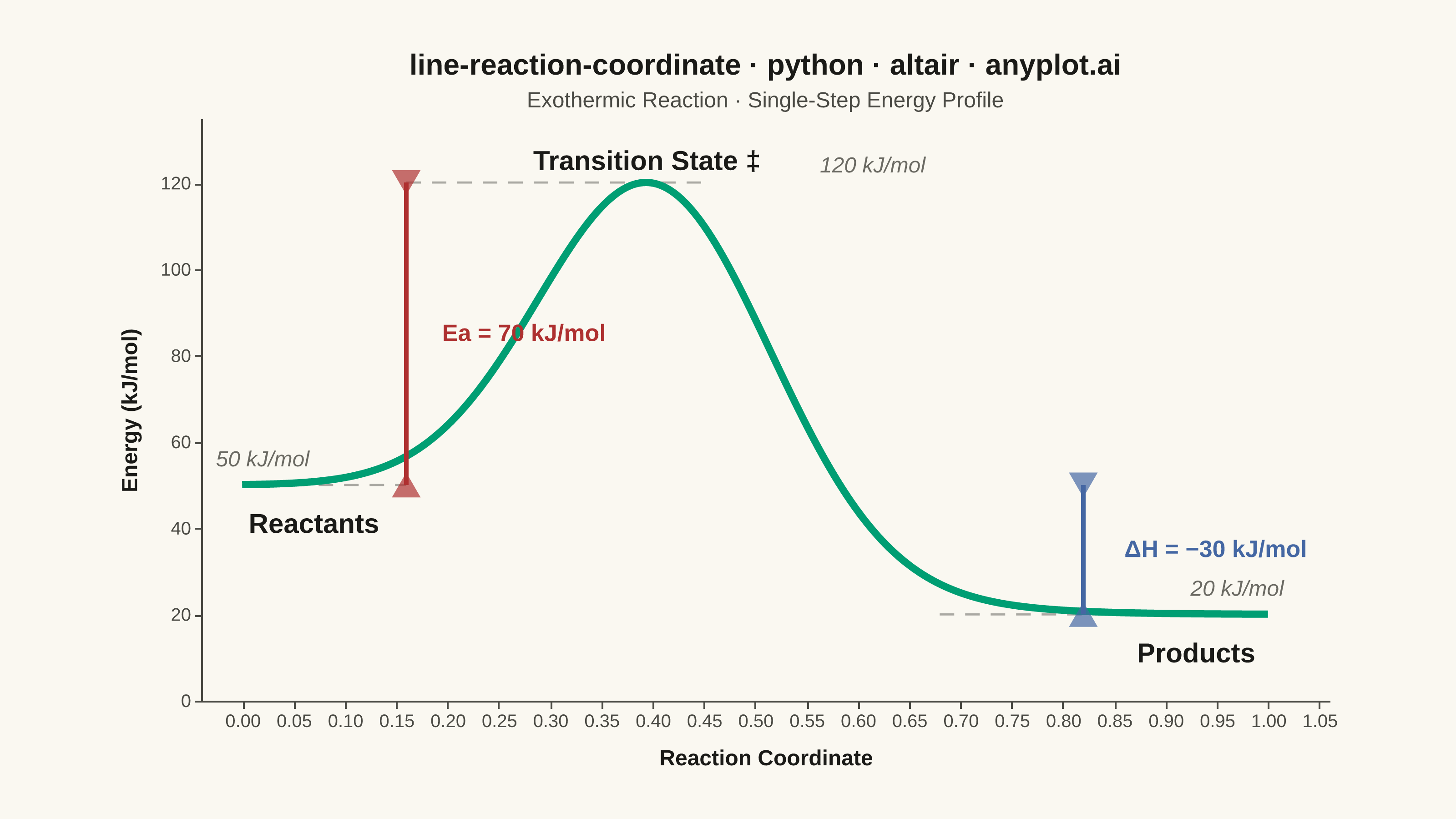
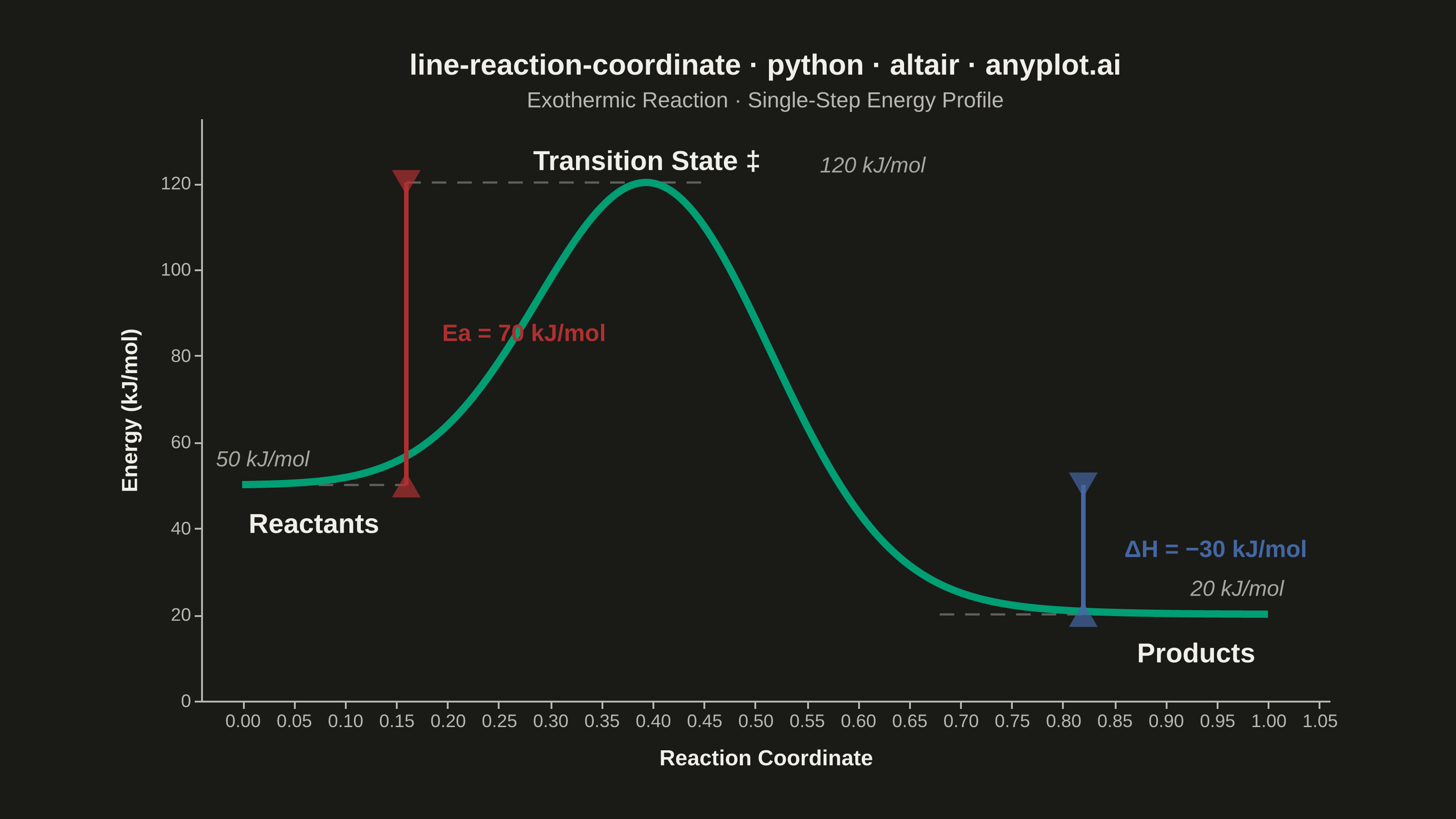
A reaction coordinate diagram plots potential energy against reaction progress, showing the energy landscape of a chemical transformation. The smooth curve traces the path from reactants through the transition state (energy maximum) to products, clearly depicting the activation energy barrier and overall enthalpy change. This fundamental chemistry visualization is essential for understanding reaction kinetics and thermodynamics.
""" anyplot.ai
line-reaction-coordinate: Reaction Coordinate Energy Diagram
Library: altair 6.2.2 | Python 3.13.14
Quality: 93/100 | Updated: 2026-06-24
"""

import os

import altair as alt
import numpy as np
import pandas as pd
from PIL import Image


# Theme tokens
THEME = os.getenv("ANYPLOT_THEME", "light")
PAGE_BG = "#FAF8F1" if THEME == "light" else "#1A1A17"
INK = "#1A1A17" if THEME == "light" else "#F0EFE8"
INK_SOFT = "#4A4A44" if THEME == "light" else "#B8B7B0"
INK_MUTED = "#6B6A63" if THEME == "light" else "#A8A79F"

# Imprint palette
curve_color = "#009E73"  # brand green — first Imprint position
ea_color = "#AE3030"  # matte red — semantic for activation barrier/cost
dh_color = "#4467A3"  # blue — third Imprint position

# Data — single-step exothermic reaction
reactant_energy = 50.0  # kJ/mol
transition_energy = 120.0  # kJ/mol
product_energy = 20.0  # kJ/mol

reaction_coord = np.linspace(0, 1, 300)
peak_pos = 0.40
sigma = 0.11

baseline = reactant_energy + (product_energy - reactant_energy) / (1 + np.exp(-14 * (reaction_coord - 0.55)))
gaussian = np.exp(-((reaction_coord - peak_pos) ** 2) / (2 * sigma**2))
baseline_at_peak = reactant_energy + (product_energy - reactant_energy) / (1 + np.exp(-14 * (peak_pos - 0.55)))
bump_height = transition_energy - baseline_at_peak
energy = baseline + bump_height * gaussian

curve_df = pd.DataFrame({"x": reaction_coord, "y": energy})
peak_idx = int(np.argmax(energy))
actual_peak_energy = float(energy[peak_idx])
peak_x = float(reaction_coord[peak_idx])
ea_value = actual_peak_energy - reactant_energy
dh_value = reactant_energy - product_energy

ea_x = 0.16
dh_x = 0.82

# Reference line data (dashed horizontal lines at each energy level)
hlines_df = pd.DataFrame(
    {
        "x": [0.0, ea_x, ea_x, peak_x + 0.06, 0.68, 1.0],
        "y": [reactant_energy, reactant_energy, actual_peak_energy, actual_peak_energy, product_energy, product_energy],
        "group": ["reactant", "reactant", "ts", "ts", "product", "product"],
    }
)

# Shared axis scales
x_scale = alt.Scale(domain=[-0.04, 1.06], nice=False)
y_scale = alt.Scale(domain=[0, 135])

# Energy curve
curve = (
    alt.Chart(curve_df)
    .mark_line(strokeWidth=4, color=curve_color)
    .encode(
        x=alt.X("x:Q", scale=x_scale, title="Reaction Coordinate"),
        y=alt.Y("y:Q", scale=y_scale, title="Energy (kJ/mol)"),
        tooltip=[
            alt.Tooltip("x:Q", title="Reaction Coordinate", format=".2f"),
            alt.Tooltip("y:Q", title="Energy (kJ/mol)", format=".1f"),
        ],
    )
)

# Dashed reference lines at each energy level
hlines = (
    alt.Chart(hlines_df)
    .mark_line(strokeWidth=1.2, strokeDash=[8, 6], color=INK_SOFT, opacity=0.45)
    .encode(x=alt.X("x:Q", scale=x_scale), y=alt.Y("y:Q", scale=y_scale), detail="group:N")
)

# Activation energy (Ea) double-headed arrow
ea_line = (
    alt.Chart(pd.DataFrame({"x": [ea_x, ea_x], "y": [reactant_energy, actual_peak_energy]}))
    .mark_line(strokeWidth=2.5, color=ea_color)
    .encode(x=alt.X("x:Q", scale=x_scale), y=alt.Y("y:Q", scale=y_scale))
)
ea_heads = (
    alt.Chart(
        pd.DataFrame(
            {"x": [ea_x, ea_x], "y": [actual_peak_energy, reactant_energy], "shape": ["triangle-up", "triangle-down"]}
        )
    )
    .mark_point(filled=True, size=250, color=ea_color)
    .encode(
        x=alt.X("x:Q", scale=x_scale),
        y=alt.Y("y:Q", scale=y_scale),
        shape=alt.Shape("shape:N", scale=alt.Scale(range=["triangle-up", "triangle-down"]), legend=None),
    )
)

# Enthalpy change (ΔH) double-headed arrow
dh_line = (
    alt.Chart(pd.DataFrame({"x": [dh_x, dh_x], "y": [product_energy, reactant_energy]}))
    .mark_line(strokeWidth=2.5, color=dh_color)
    .encode(x=alt.X("x:Q", scale=x_scale), y=alt.Y("y:Q", scale=y_scale))
)
dh_heads = (
    alt.Chart(
        pd.DataFrame(
            {"x": [dh_x, dh_x], "y": [reactant_energy, product_energy], "shape": ["triangle-up", "triangle-down"]}
        )
    )
    .mark_point(filled=True, size=250, color=dh_color)
    .encode(
        x=alt.X("x:Q", scale=x_scale),
        y=alt.Y("y:Q", scale=y_scale),
        shape=alt.Shape("shape:N", scale=alt.Scale(range=["triangle-up", "triangle-down"]), legend=None),
    )
)

# Species labels
species_df = pd.DataFrame(
    {
        "x": [0.07, peak_x, 0.93],
        "y": [reactant_energy - 9, actual_peak_energy + 5, product_energy - 9],
        "text": ["Reactants", "Transition State ‡", "Products"],
    }
)
species_labels = (
    alt.Chart(species_df)
    .mark_text(fontSize=15, fontWeight="bold", color=INK)
    .encode(x=alt.X("x:Q", scale=x_scale), y=alt.Y("y:Q", scale=y_scale), text="text:N")
)

# Arrow value labels (Ea and ΔH magnitudes)
arrow_labels_df = pd.DataFrame(
    {
        "x": [ea_x + 0.035, dh_x + 0.04],
        "y": [(reactant_energy + actual_peak_energy) / 2, (reactant_energy + product_energy) / 2],
        "text": [f"Ea = {ea_value:.0f} kJ/mol", f"ΔH = −{dh_value:.0f} kJ/mol"],
        "color": [ea_color, dh_color],
    }
)
arrow_labels = (
    alt.Chart(arrow_labels_df)
    .mark_text(fontSize=13, fontWeight="bold", align="left")
    .encode(
        x=alt.X("x:Q", scale=x_scale),
        y=alt.Y("y:Q", scale=y_scale),
        text="text:N",
        color=alt.Color("color:N", scale=None),
    )
)

# Energy level value annotations (muted, italic)
energy_vals_df = pd.DataFrame(
    {
        "x": [0.02, 0.97, peak_x + 0.22],
        "y": [reactant_energy + 6, product_energy + 6, actual_peak_energy + 4],
        "text": [f"{reactant_energy:.0f} kJ/mol", f"{product_energy:.0f} kJ/mol", f"{actual_peak_energy:.0f} kJ/mol"],
    }
)
energy_vals = (
    alt.Chart(energy_vals_df)
    .mark_text(fontSize=12, fontStyle="italic", color=INK_MUTED)
    .encode(x=alt.X("x:Q", scale=x_scale), y=alt.Y("y:Q", scale=y_scale), text="text:N")
)

# Title (55 chars < 67 baseline, no scaling needed)
title_str = "line-reaction-coordinate · python · altair · anyplot.ai"

# Combine all layers and apply theme-adaptive chrome
chart = (
    alt.layer(hlines, curve, ea_line, ea_heads, dh_line, dh_heads, species_labels, arrow_labels, energy_vals)
    .properties(
        background=PAGE_BG,
        width=620,
        height=320,
        title=alt.Title(
            title_str,
            fontSize=16,
            anchor="middle",
            color=INK,
            subtitle="Exothermic Reaction · Single-Step Energy Profile",
            subtitleFontSize=12,
            subtitleColor=INK_SOFT,
            subtitlePadding=6,
        ),
    )
    .configure_view(fill=PAGE_BG, strokeWidth=0)
    .configure_axis(
        labelFontSize=10,
        titleFontSize=12,
        titleColor=INK,
        labelColor=INK_SOFT,
        domainColor=INK_SOFT,
        tickColor=INK_SOFT,
        tickSize=4,
        titlePadding=10,
        grid=False,
    )
    .configure_title(color=INK)
    .interactive()
)

# Save — pad PNG to exact 3200×1800 target
TW, TH = 3200, 1800

chart.save(f"plot-{THEME}.png", scale_factor=4.0)

_img = Image.open(f"plot-{THEME}.png").convert("RGB")
_w, _h = _img.size
if _w > TW or _h > TH:
    raise SystemExit(
        f"altair vl-convert produced {_w}×{_h}, exceeds target {TW}×{TH}. "
        f"Shrink chart .properties(width=, height=) values and re-render."
    )
if _w < TW or _h < TH:
    _canvas = Image.new("RGB", (TW, TH), PAGE_BG)
    _canvas.paste(_img, ((TW - _w) // 2, (TH - _h) // 2))
    _canvas.save(f"plot-{THEME}.png")

chart.save(f"plot-{THEME}.html")
Runnable source as JSON, for any HTTP client: https://api.anyplot.ai/specs/line-reaction-coordinate/altair/code. Any spec id and library id listed in llms-full.txt fit the same URL shape; every URL below is complete and callable.
{
  "spec_id": "line-reaction-coordinate",
  "language": "python",
  "library": "altair",
  "page": "https://anyplot.ai/line-reaction-coordinate/python/altair",
  "hub": "https://anyplot.ai/line-reaction-coordinate",
  "code_json": "https://api.anyplot.ai/specs/line-reaction-coordinate/altair/code",
  "spec_json": "https://api.anyplot.ai/specs/line-reaction-coordinate",
  "render_light_png": "https://storage.googleapis.com/anyplot-images/plots/line-reaction-coordinate/python/altair/plot-light.png",
  "render_dark_png": "https://storage.googleapis.com/anyplot-images/plots/line-reaction-coordinate/python/altair/plot-dark.png",
  "interactive_light_html": "https://storage.googleapis.com/anyplot-images/plots/line-reaction-coordinate/python/altair/plot-light.html",
  "interactive_dark_html": "https://storage.googleapis.com/anyplot-images/plots/line-reaction-coordinate/python/altair/plot-dark.html",
  "quality_score": 93.0,
  "license": "MIT",
  "guide": "https://anyplot.ai/llms.txt"
}
Part of Reaction Coordinate Energy Diagram on anyplot.ai.