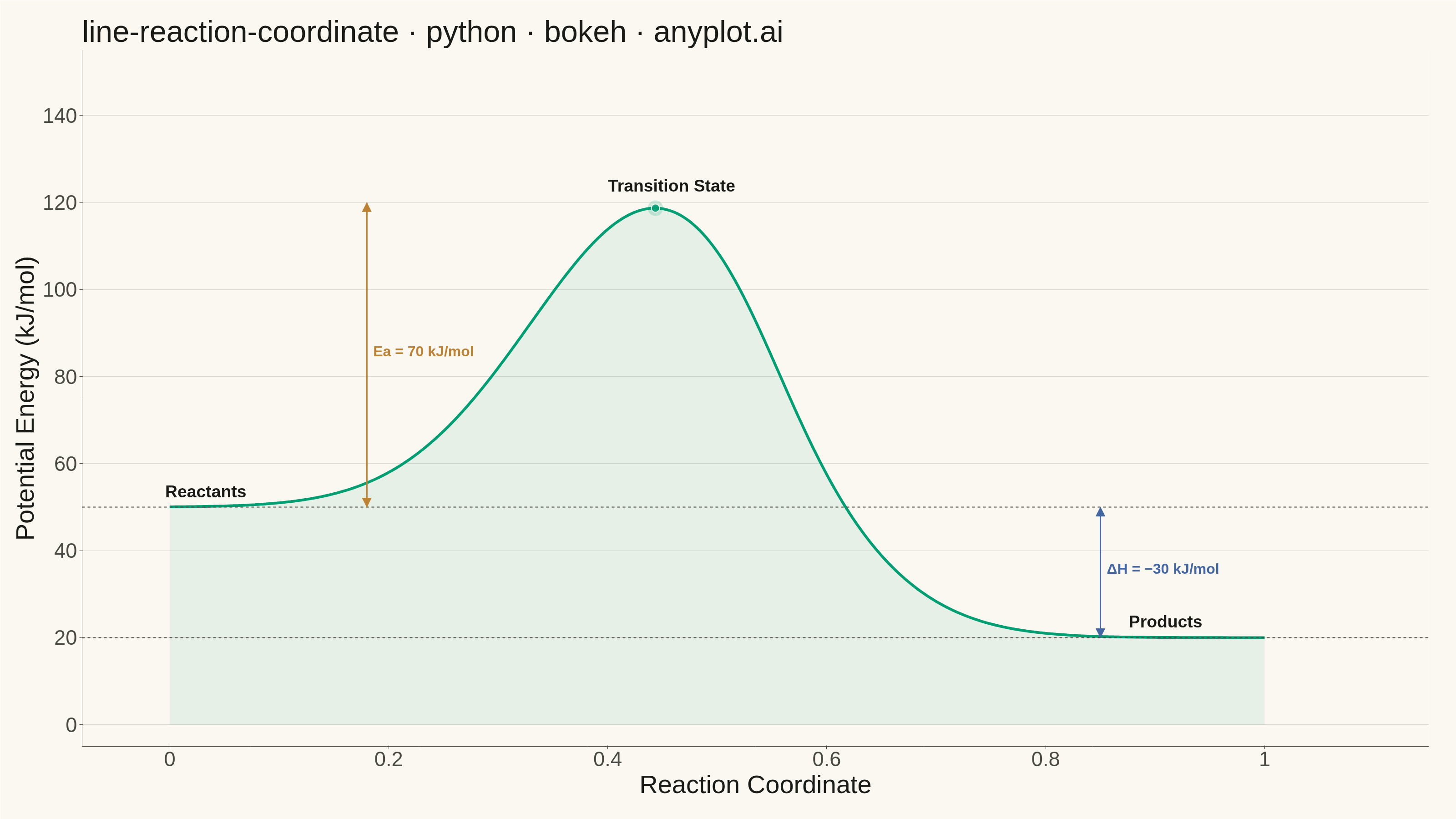
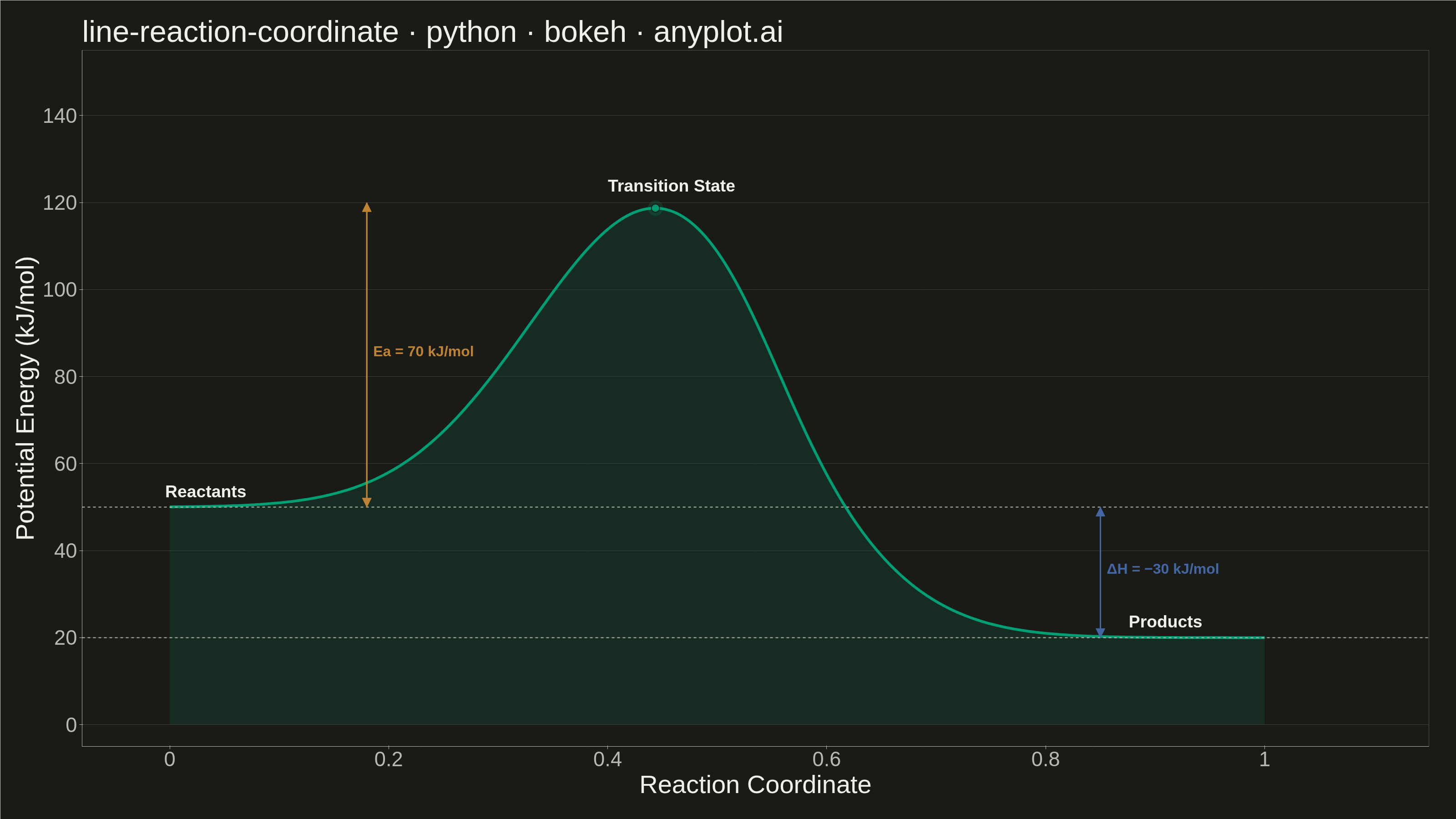
A reaction coordinate diagram plots potential energy against reaction progress, showing the energy landscape of a chemical transformation. The smooth curve traces the path from reactants through the transition state (energy maximum) to products, clearly depicting the activation energy barrier and overall enthalpy change. This fundamental chemistry visualization is essential for understanding reaction kinetics and thermodynamics.
""" anyplot.ai
line-reaction-coordinate: Reaction Coordinate Energy Diagram
Library: bokeh 3.9.1 | Python 3.13.14
Quality: 90/100 | Updated: 2026-06-24
"""

import io
import os
import sys
import time
from pathlib import Path


# Prevent this file's directory from shadowing the installed bokeh package
sys.path = [p for p in sys.path if os.path.abspath(p) != os.path.dirname(os.path.abspath(__file__))]

import numpy as np
from bokeh.io import output_file, save
from bokeh.models import Arrow, ColumnDataSource, Label, NormalHead, Span
from bokeh.plotting import figure
from PIL import Image
from selenium import webdriver
from selenium.webdriver.chrome.options import Options


# Theme tokens
THEME = os.getenv("ANYPLOT_THEME", "light")
PAGE_BG = "#FAF8F1" if THEME == "light" else "#1A1A17"
ELEVATED_BG = "#FFFDF6" if THEME == "light" else "#242420"
INK = "#1A1A17" if THEME == "light" else "#F0EFE8"
INK_SOFT = "#4A4A44" if THEME == "light" else "#B8B7B0"
INK_MUTED = "#6B6A63" if THEME == "light" else "#A8A79F"

# Imprint palette — positions used for annotation arrows
BRAND = "#009E73"  # Imprint position 1 — main energy curve
EA_COLOR = "#BD8233"  # Imprint position 4 — activation energy arrow
DH_COLOR = "#4467A3"  # Imprint position 3 — enthalpy change arrow

# Data
reactant_energy = 50.0
transition_energy = 120.0
product_energy = 20.0

reaction_coord = np.linspace(0, 1, 400)

peak_center = 0.45
peak_width = 0.12
gaussian_peak = (transition_energy - reactant_energy) * np.exp(
    -((reaction_coord - peak_center) ** 2) / (2 * peak_width**2)
)

sigmoid = 1 / (1 + np.exp(30 * (reaction_coord - 0.55)))
baseline = reactant_energy * sigmoid + product_energy * (1 - sigmoid)

energy = baseline + gaussian_peak

source = ColumnDataSource(data={"x": reaction_coord, "y": energy})

# Title — 54 chars, under the 67-char baseline so no font scaling needed
TITLE = "line-reaction-coordinate · python · bokeh · anyplot.ai"

# Plot
p = figure(
    width=3200,
    height=1800,
    title=TITLE,
    x_axis_label="Reaction Coordinate",
    y_axis_label="Potential Energy (kJ/mol)",
    x_range=(-0.08, 1.15),
    y_range=(-5, 155),
    toolbar_location=None,
    min_border_bottom=160,
    min_border_left=180,
    min_border_top=110,
    min_border_right=60,
)

# Area fill under the energy curve — slightly stronger in dark mode for visibility
fill_alpha = 0.08 if THEME == "light" else 0.14
p.varea(x="x", y1=0, y2="y", source=source, fill_color=BRAND, fill_alpha=fill_alpha)

# Main energy curve
p.line("x", "y", source=source, line_width=6, color=BRAND)

# Transition state emphasis
ts_idx = int(np.argmax(energy))
ts_x_val = float(reaction_coord[ts_idx])
ts_y_val = float(energy[ts_idx])
p.scatter([ts_x_val], [ts_y_val], size=34, color=BRAND, alpha=0.18, line_color=None)
p.scatter([ts_x_val], [ts_y_val], size=18, color=BRAND, alpha=0.9, line_color=PAGE_BG, line_width=2)

# Horizontal dashed reference lines at reactant and product levels
p.add_layout(Span(location=reactant_energy, dimension="width", line_color=INK_SOFT, line_width=2, line_dash="dashed"))
p.add_layout(Span(location=product_energy, dimension="width", line_color=INK_SOFT, line_width=2, line_dash="dashed"))

# State labels
state_kwargs = {"text_font_size": "28pt", "text_color": INK, "text_font_style": "bold"}
p.add_layout(Label(x=0.0, y=reactant_energy, text="Reactants", x_offset=-10, y_offset=14, **state_kwargs))
p.add_layout(Label(x=0.88, y=product_energy, text="Products", x_offset=-10, y_offset=14, **state_kwargs))
p.add_layout(
    Label(x=peak_center, y=transition_energy, text="Transition State", x_offset=-120, y_offset=16, **state_kwargs)
)

# Activation energy (Eₐ) double-headed arrows
ea_x = 0.18
head_size = 20
p.add_layout(
    Arrow(
        end=NormalHead(size=head_size, fill_color=EA_COLOR, line_color=EA_COLOR),
        x_start=ea_x,
        y_start=reactant_energy,
        x_end=ea_x,
        y_end=transition_energy,
        line_color=EA_COLOR,
        line_width=3,
    )
)
p.add_layout(
    Arrow(
        end=NormalHead(size=head_size, fill_color=EA_COLOR, line_color=EA_COLOR),
        x_start=ea_x,
        y_start=transition_energy,
        x_end=ea_x,
        y_end=reactant_energy,
        line_color=EA_COLOR,
        line_width=3,
    )
)
p.add_layout(
    Label(
        x=ea_x,
        y=(reactant_energy + transition_energy) / 2,
        text="Ea = 70 kJ/mol",
        text_font_size="24pt",
        text_color=EA_COLOR,
        text_font_style="bold",
        x_offset=14,
        y_offset=-10,
    )
)

# Enthalpy change (ΔH) double-headed arrows
dh_x = 0.85
p.add_layout(
    Arrow(
        end=NormalHead(size=head_size, fill_color=DH_COLOR, line_color=DH_COLOR),
        x_start=dh_x,
        y_start=product_energy,
        x_end=dh_x,
        y_end=reactant_energy,
        line_color=DH_COLOR,
        line_width=3,
    )
)
p.add_layout(
    Arrow(
        end=NormalHead(size=head_size, fill_color=DH_COLOR, line_color=DH_COLOR),
        x_start=dh_x,
        y_start=reactant_energy,
        x_end=dh_x,
        y_end=product_energy,
        line_color=DH_COLOR,
        line_width=3,
    )
)
p.add_layout(
    Label(
        x=dh_x,
        y=(reactant_energy + product_energy) / 2,
        text="ΔH = −30 kJ/mol",
        text_font_size="24pt",
        text_color=DH_COLOR,
        text_font_style="bold",
        x_offset=14,
        y_offset=-10,
    )
)

# Theme-adaptive chrome
p.title.text_font_size = "50pt"
p.title.text_color = INK
p.title.text_font_style = "normal"

p.xaxis.axis_label_text_font_size = "42pt"
p.yaxis.axis_label_text_font_size = "42pt"
p.xaxis.axis_label_text_font_style = "normal"
p.yaxis.axis_label_text_font_style = "normal"
p.xaxis.major_label_text_font_size = "34pt"
p.yaxis.major_label_text_font_size = "34pt"
p.xaxis.axis_label_text_color = INK
p.yaxis.axis_label_text_color = INK
p.xaxis.major_label_text_color = INK_SOFT
p.yaxis.major_label_text_color = INK_SOFT
p.xaxis.axis_line_color = INK_SOFT
p.yaxis.axis_line_color = INK_SOFT
p.xaxis.major_tick_line_color = INK_SOFT
p.yaxis.major_tick_line_color = INK_SOFT
p.xaxis.minor_tick_line_color = None
p.yaxis.minor_tick_line_color = None

p.xgrid.grid_line_color = None
p.ygrid.grid_line_color = INK
p.ygrid.grid_line_alpha = 0.15

p.background_fill_color = PAGE_BG
p.border_fill_color = PAGE_BG
p.outline_line_color = None

# Save HTML (interactive catalog artifact)
output_file(f"plot-{THEME}.html")
save(p)

# Screenshot with headless Chrome (Selenium 4 / Selenium Manager).
# Chrome's internal UI overhead shrinks the viewport below --window-size by ~139 px.
# Use a taller window (H + 200 buffer) so the viewport is >= H, then crop to exact dims.
W, H = 3200, 1800
opts = Options()
for arg in (
    "--headless=new",
    "--no-sandbox",
    "--disable-dev-shm-usage",
    "--disable-gpu",
    f"--window-size={W},{H + 200}",
    "--hide-scrollbars",
    "--force-device-scale-factor=1",
):
    opts.add_argument(arg)
driver = webdriver.Chrome(options=opts)
driver.set_window_size(W, H + 200)
driver.get(f"file://{Path(f'plot-{THEME}.html').resolve()}")
time.sleep(3)
raw = driver.get_screenshot_as_png()
driver.quit()
img = Image.open(io.BytesIO(raw)).crop((0, 0, W, H))
img.save(f"plot-{THEME}.png")
Runnable source as JSON, for any HTTP client: https://api.anyplot.ai/specs/line-reaction-coordinate/bokeh/code. Any spec id and library id listed in llms-full.txt fit the same URL shape; every URL below is complete and callable.
{
  "spec_id": "line-reaction-coordinate",
  "language": "python",
  "library": "bokeh",
  "page": "https://anyplot.ai/line-reaction-coordinate/python/bokeh",
  "hub": "https://anyplot.ai/line-reaction-coordinate",
  "code_json": "https://api.anyplot.ai/specs/line-reaction-coordinate/bokeh/code",
  "spec_json": "https://api.anyplot.ai/specs/line-reaction-coordinate",
  "render_light_png": "https://storage.googleapis.com/anyplot-images/plots/line-reaction-coordinate/python/bokeh/plot-light.png",
  "render_dark_png": "https://storage.googleapis.com/anyplot-images/plots/line-reaction-coordinate/python/bokeh/plot-dark.png",
  "interactive_light_html": "https://storage.googleapis.com/anyplot-images/plots/line-reaction-coordinate/python/bokeh/plot-light.html",
  "interactive_dark_html": "https://storage.googleapis.com/anyplot-images/plots/line-reaction-coordinate/python/bokeh/plot-dark.html",
  "quality_score": 90.0,
  "license": "MIT",
  "guide": "https://anyplot.ai/llms.txt"
}
Part of Reaction Coordinate Energy Diagram on anyplot.ai.