The same plot in 14 other libraries — Python: Altair, Bokeh, lets-plot, Matplotlib, Plotly, plotnine, Pygal, Seaborn; Julia: Makie.jl; JavaScript: Chart.js, D3.js, Apache ECharts, Highcharts, MUI X Charts. Compare all 15 side by side: Reaction Coordinate Energy Diagram in Python, R, Julia and JavaScript.
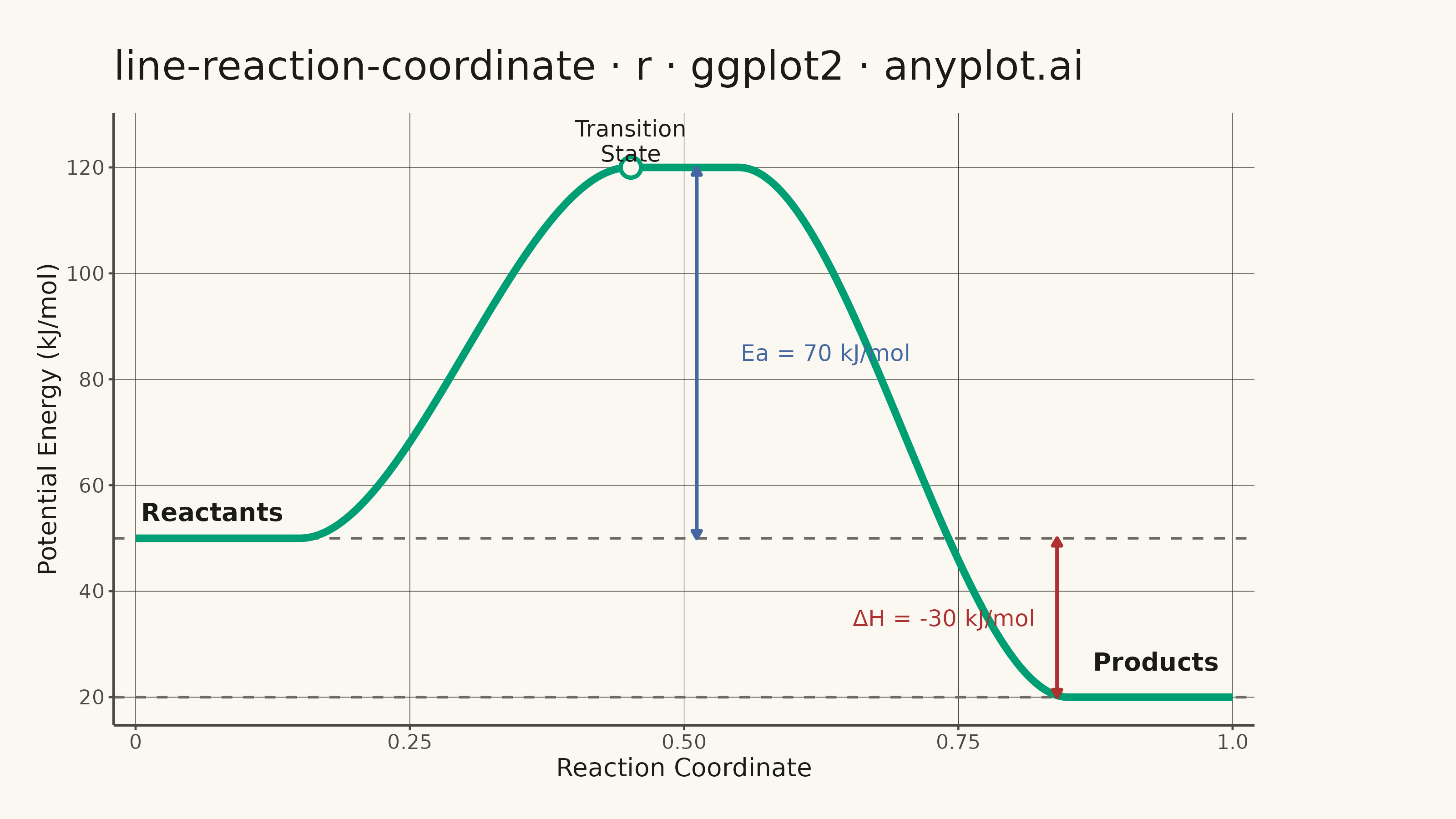
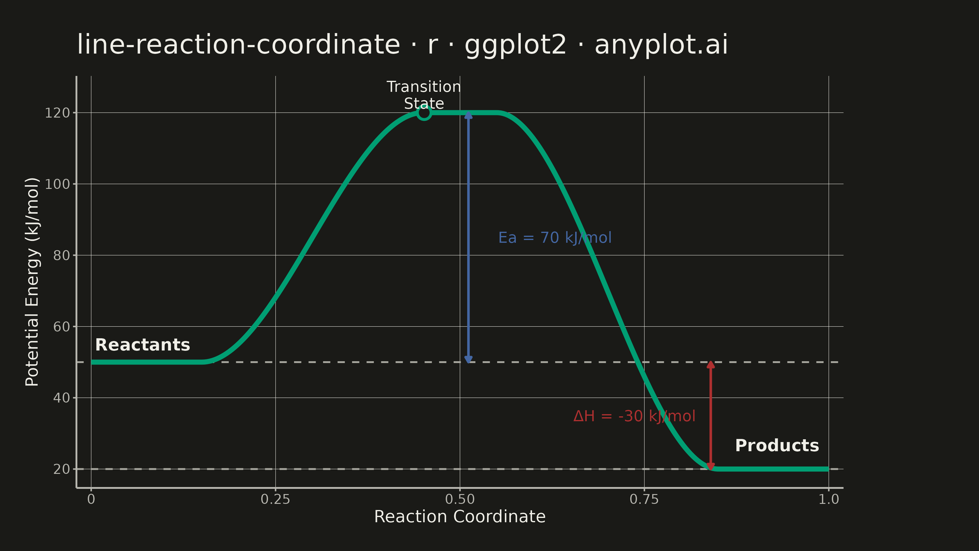
A reaction coordinate diagram plots potential energy against reaction progress, showing the energy landscape of a chemical transformation. The smooth curve traces the path from reactants through the transition state (energy maximum) to products, clearly depicting the activation energy barrier and overall enthalpy change. This fundamental chemistry visualization is essential for understanding reaction kinetics and thermodynamics.
#' anyplot.ai
#' line-reaction-coordinate: Reaction Coordinate Energy Diagram
#' Library: ggplot2 3.5.1 | R 4.4.1
#' Quality: 90/100 | Created: 2026-06-24

library(ggplot2)
library(ragg)

set.seed(42)

# Theme tokens
THEME       <- Sys.getenv("ANYPLOT_THEME", "light")
PAGE_BG     <- if (THEME == "light") "#FAF8F1" else "#1A1A17"
ELEVATED_BG <- if (THEME == "light") "#FFFDF6" else "#242420"
INK         <- if (THEME == "light") "#1A1A17" else "#F0EFE8"
INK_SOFT    <- if (THEME == "light") "#4A4A44" else "#B8B7B0"
INK_MUTED   <- if (THEME == "light") "#6B6A63" else "#A8A79F"
IMPRINT_PALETTE <- c(
  "#009E73", "#C475FD", "#4467A3", "#BD8233",
  "#AE3030", "#2ABCCD", "#954477", "#99B314"
)

# Data: single-step exothermic reaction energy curve
# Reactants at 50 kJ/mol, transition state at 120 kJ/mol, products at 20 kJ/mol
reaction_x <- seq(0, 1, length.out = 300)

# Build smooth curve via cubic spline through key points
key_x <- c(0, 0.15, 0.45, 0.55, 0.85, 1.0)
key_e <- c(50, 50, 120, 120, 20, 20)
spl   <- splinefun(key_x, key_e, method = "monoH.FC")
energy_vals <- spl(reaction_x)

df <- data.frame(x = reaction_x, energy = energy_vals)

# Key reference levels
e_reactant   <- 50
e_ts         <- 120
e_product    <- 20
x_ts         <- reaction_x[which.max(energy_vals)]
ea           <- e_ts - e_reactant   # 70 kJ/mol
delta_h      <- e_product - e_reactant  # -30 kJ/mol

# Title length scaling
plot_title  <- "line-reaction-coordinate · r · ggplot2 · anyplot.ai"
n_chars     <- nchar(plot_title)
base_size   <- 12
title_size  <- max(8, round(base_size * 67 / n_chars))

# Plot
p <- ggplot(df, aes(x = x, y = energy)) +
  # Dashed reference lines for reactant and product energy levels
  geom_hline(yintercept = e_reactant, linetype = "dashed",
             color = INK_MUTED, linewidth = 0.5) +
  geom_hline(yintercept = e_product, linetype = "dashed",
             color = INK_MUTED, linewidth = 0.5) +
  # Main energy curve
  geom_line(color = IMPRINT_PALETTE[1], linewidth = 1.4) +
  # Transition state peak marker
  annotate("point",
           x = x_ts, y = e_ts,
           color = IMPRINT_PALETTE[1], size = 3, shape = 21,
           fill = PAGE_BG, stroke = 1.2) +
  # Activation energy arrow (Ea): vertical from reactant level to TS peak
  annotate("segment",
           x = x_ts + 0.06, xend = x_ts + 0.06,
           y = e_reactant, yend = e_ts,
           arrow = arrow(ends = "both", length = unit(0.12, "cm"),
                         type = "closed"),
           color = IMPRINT_PALETTE[3], linewidth = 0.7) +
  annotate("text",
           x = x_ts + 0.10, y = (e_reactant + e_ts) / 2,
           label = paste0("Ea = ", ea, " kJ/mol"),
           color = IMPRINT_PALETTE[3], size = 3.2, hjust = 0) +
  # ΔH arrow: vertical from reactant level to product level
  annotate("segment",
           x = 0.84, xend = 0.84,
           y = e_reactant, yend = e_product,
           arrow = arrow(ends = "both", length = unit(0.12, "cm"),
                         type = "closed"),
           color = IMPRINT_PALETTE[5], linewidth = 0.7) +
  annotate("text",
           x = 0.82, y = (e_reactant + e_product) / 2,
           label = paste0("ΔH = ", delta_h, " kJ/mol"),
           color = IMPRINT_PALETTE[5], size = 3.2, hjust = 1) +
  # Labels: Reactants, Transition State, Products
  annotate("text",
           x = 0.07, y = e_reactant + 5,
           label = "Reactants", color = INK, size = 3.5, fontface = "bold",
           hjust = 0.5) +
  annotate("text",
           x = x_ts, y = e_ts + 5,
           label = "Transition\nState", color = INK, size = 3.2,
           hjust = 0.5, lineheight = 0.9) +
  annotate("text",
           x = 0.93, y = e_product + 5,
           label = "Products", color = INK, size = 3.5, fontface = "bold",
           hjust = 0.5, vjust = 0) +
  labs(
    title = plot_title,
    x     = "Reaction Coordinate",
    y     = "Potential Energy (kJ/mol)"
  ) +
  scale_x_continuous(
    breaks = c(0, 0.25, 0.5, 0.75, 1.0),
    labels = c("0", "0.25", "0.50", "0.75", "1.0"),
    expand = c(0.01, 0.01)
  ) +
  scale_y_continuous(
    breaks = seq(0, 130, by = 20),
    expand = c(0.05, 0.05)
  ) +
  theme_minimal(base_size = 8) +
  theme(
    plot.background   = element_rect(fill = PAGE_BG, color = PAGE_BG),
    panel.background  = element_rect(fill = PAGE_BG, color = NA),
    panel.grid.major  = element_line(color = INK, linewidth = 0.10),
    panel.grid.minor  = element_blank(),
    panel.border      = element_blank(),
    axis.line         = element_line(color = INK_SOFT, linewidth = 0.5),
    axis.ticks        = element_line(color = INK_SOFT, linewidth = 0.4),
    axis.title        = element_text(color = INK, size = 10),
    axis.text         = element_text(color = INK_SOFT, size = 8),
    plot.title        = element_text(color = INK, size = title_size,
                                     margin = margin(b = 10)),
    plot.margin       = margin(t = 20, r = 80, b = 15, l = 15)
  )

# Save
ggsave(
  filename = sprintf("plot-%s.png", THEME),
  plot     = p,
  device   = ragg::agg_png,
  width    = 8,
  height   = 4.5,
  units    = "in",
  dpi      = 400
)
Runnable source as JSON, for any HTTP client: https://api.anyplot.ai/specs/line-reaction-coordinate/ggplot2/code. Any spec id and library id listed in llms-full.txt fit the same URL shape; every URL below is complete and callable.
{
  "spec_id": "line-reaction-coordinate",
  "language": "r",
  "library": "ggplot2",
  "page": "https://anyplot.ai/line-reaction-coordinate/r/ggplot2",
  "hub": "https://anyplot.ai/line-reaction-coordinate",
  "code_json": "https://api.anyplot.ai/specs/line-reaction-coordinate/ggplot2/code",
  "spec_json": "https://api.anyplot.ai/specs/line-reaction-coordinate",
  "render_light_png": "https://storage.googleapis.com/anyplot-images/plots/line-reaction-coordinate/r/ggplot2/plot-light.png",
  "render_dark_png": "https://storage.googleapis.com/anyplot-images/plots/line-reaction-coordinate/r/ggplot2/plot-dark.png",
  "quality_score": 90.0,
  "license": "MIT",
  "guide": "https://anyplot.ai/llms.txt"
}
Part of Reaction Coordinate Energy Diagram on anyplot.ai.