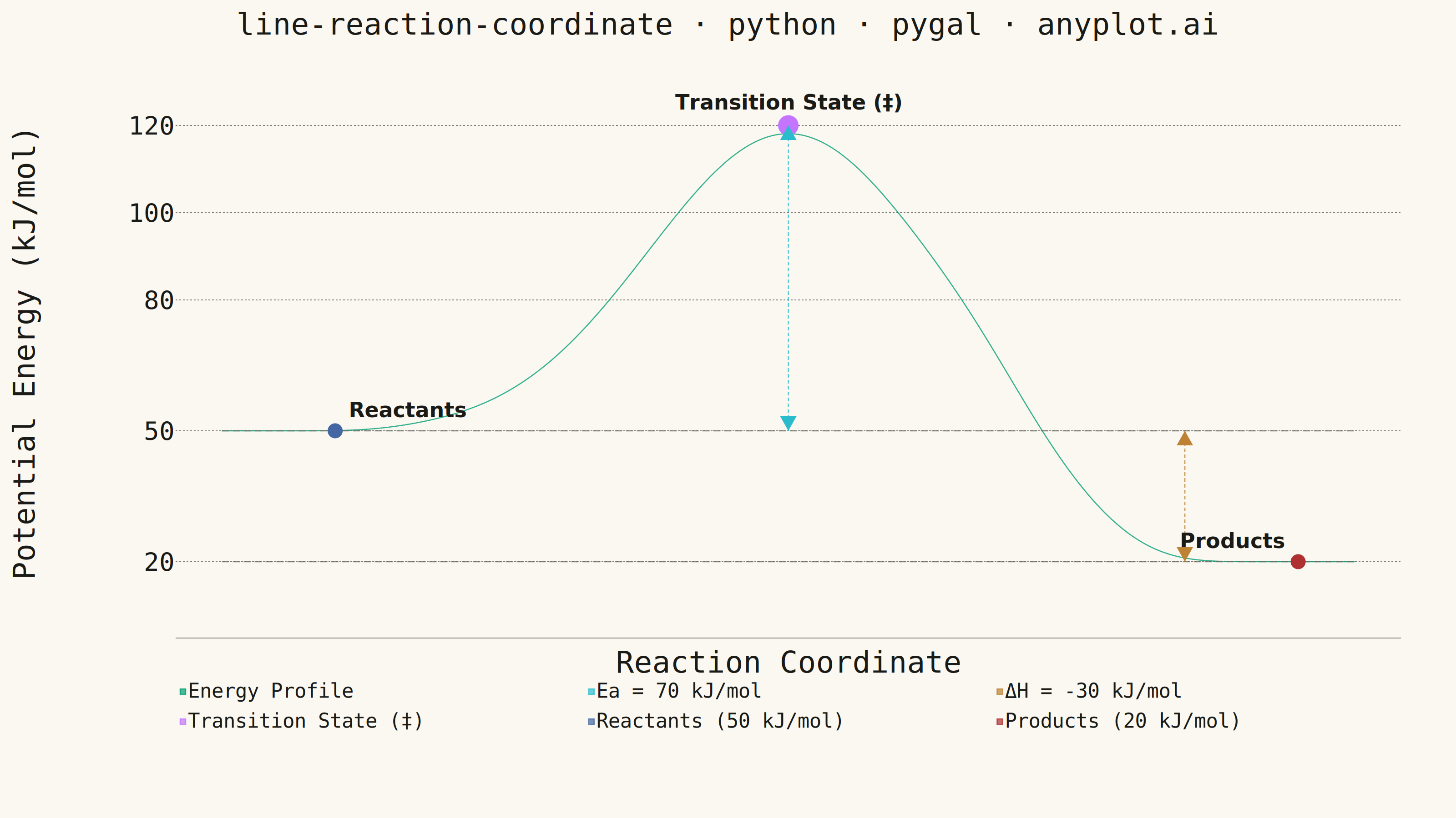
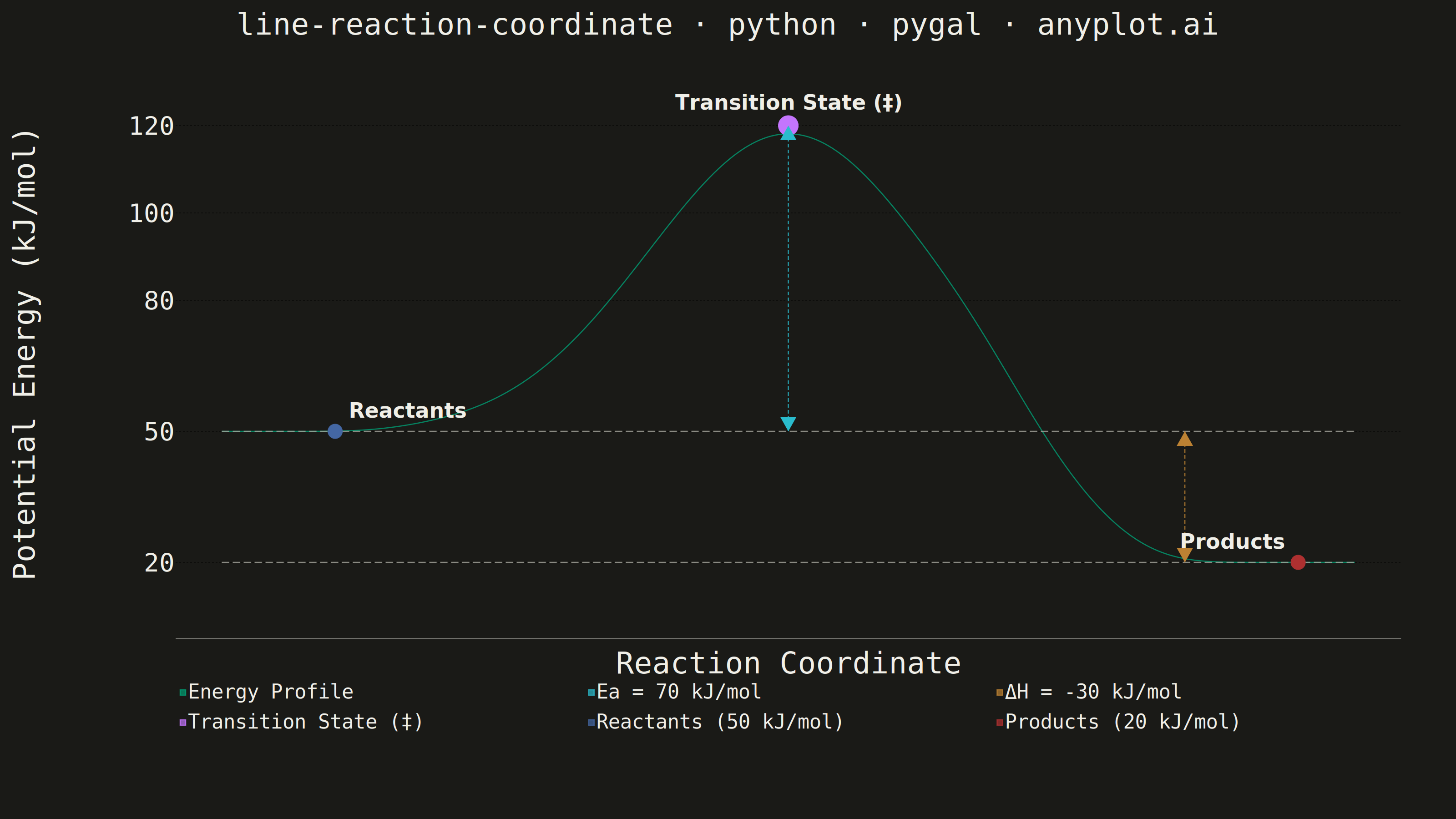
A reaction coordinate diagram plots potential energy against reaction progress, showing the energy landscape of a chemical transformation. The smooth curve traces the path from reactants through the transition state (energy maximum) to products, clearly depicting the activation energy barrier and overall enthalpy change. This fundamental chemistry visualization is essential for understanding reaction kinetics and thermodynamics.
""" anyplot.ai
line-reaction-coordinate: Reaction Coordinate Energy Diagram
Library: pygal 3.1.3 | Python 3.13.14
Quality: 87/100 | Updated: 2026-06-24
"""

import os
import re
import sys


# Script filename shadows the installed 'pygal' package when run as 'python pygal.py';
# dropping the script directory from sys.path lets the real package resolve.
sys.path.pop(0)

import cairosvg
import numpy as np
import pygal
from pygal.style import Style


# Theme tokens — Imprint palette chrome
THEME = os.getenv("ANYPLOT_THEME", "light")
PAGE_BG = "#FAF8F1" if THEME == "light" else "#1A1A17"
INK = "#1A1A17" if THEME == "light" else "#F0EFE8"
INK_MUTED = "#6B6A63" if THEME == "light" else "#A8A79F"

# Data — single-step exothermic reaction
reactant_energy = 50.0
transition_energy = 120.0
product_energy = 20.0
activation_energy = transition_energy - reactant_energy  # Ea = 70 kJ/mol
enthalpy_change = product_energy - reactant_energy  # ΔH = -30 kJ/mol

# Generate smooth energy profile
n_points = 300
reaction_coord = np.linspace(0, 10, n_points)

sigma = 1.2
peak_pos = 5.0
base_curve = reactant_energy + (transition_energy - reactant_energy) * np.exp(
    -0.5 * ((reaction_coord - peak_pos) / sigma) ** 2
)

t_raw = np.clip((reaction_coord - 6.5) / 2.0, 0.0, 1.0)
smooth_t = t_raw * t_raw * (3 - 2 * t_raw)
base_curve = base_curve * (1 - smooth_t) + product_energy * smooth_t

base_curve = np.where(reaction_coord < 1.5, reactant_energy, base_curve)
base_curve = np.where(reaction_coord > 8.5, product_energy, base_curve)

kernel = np.ones(17) / 17
energy_curve = base_curve.copy()
for _ in range(3):
    padded = np.pad(energy_curve, 17, mode="edge")
    energy_curve = np.convolve(padded, kernel, mode="same")[17:-17]

curve_points = list(zip(reaction_coord.tolist(), energy_curve.tolist(), strict=True))

# Series colors: Imprint palette positions assigned by role
EA_COLOR = "#2ABCCD"  # Ea indicator — Imprint pos 6 (cyan/teal)
DH_COLOR = "#BD8233"  # ΔH indicator — Imprint pos 4 (ochre/warm)
SERIES_COLORS = (
    "#009E73",  # Energy Profile — Imprint pos 1 (brand green)
    INK_MUTED,  # Reference line at reactant level (theme-adaptive muted)
    INK_MUTED,  # Reference line at product level (theme-adaptive muted)
    EA_COLOR,  # Ea indicator
    DH_COLOR,  # ΔH indicator
    "#C475FD",  # Transition State — Imprint pos 2 (lavender)
    "#4467A3",  # Reactants — Imprint pos 3 (blue)
    "#AE3030",  # Products — Imprint pos 5 (matte red)
)

custom_style = Style(
    background=PAGE_BG,
    plot_background=PAGE_BG,
    foreground=INK,
    foreground_strong=INK,
    foreground_subtle=INK_MUTED,
    colors=SERIES_COLORS,
    title_font_size=66,
    label_font_size=56,
    major_label_font_size=44,
    legend_font_size=44,
    value_font_size=36,
    stroke_width=2.5,
)

chart = pygal.XY(
    width=3200,
    height=1800,
    style=custom_style,
    title="line-reaction-coordinate · python · pygal · anyplot.ai",
    x_title="Reaction Coordinate",
    y_title="Potential Energy (kJ/mol)",
    show_legend=True,
    legend_at_bottom=True,
    legend_at_bottom_columns=3,
    show_x_guides=False,
    show_y_guides=True,
    show_x_labels=False,
    dots_size=0,
    stroke=True,
    margin=60,
    margin_left=200,
    margin_right=120,
    margin_bottom=200,
    margin_top=80,
    range=(5, 130),
    xrange=(-0.2, 10.2),
    truncate_legend=-1,
    tooltip_border_radius=8,
)

# Main energy curve — Imprint pos 1 (brand green)
chart.add("Energy Profile", curve_points, stroke_style={"width": 6}, show_dots=False, fill=False)

# Horizontal reference lines at key energy levels
chart.add(
    None,
    [(0.0, reactant_energy), (10.0, reactant_energy)],
    stroke_style={"width": 3, "dasharray": "16, 8"},
    show_dots=False,
)
chart.add(
    None,
    [(0.0, product_energy), (10.0, product_energy)],
    stroke_style={"width": 3, "dasharray": "16, 8"},
    show_dots=False,
)

# Ea and ΔH vertical indicators — no endpoint circles; arrowheads injected via SVG
ea_x = peak_pos
chart.add(
    f"Ea = {activation_energy:.0f} kJ/mol",
    [(ea_x, reactant_energy), (ea_x, transition_energy)],
    stroke_style={"width": 5, "dasharray": "8, 5"},
    show_dots=False,
)

dh_x = 8.5
chart.add(
    f"ΔH = {enthalpy_change:.0f} kJ/mol",
    [(dh_x, reactant_energy), (dh_x, product_energy)],
    stroke_style={"width": 5, "dasharray": "8, 5"},
    show_dots=False,
)

# Key markers
chart.add(
    "Transition State (‡)",
    [{"value": (peak_pos, transition_energy), "node": {"r": 22}}],
    stroke_style={"width": 0},
    dots_size=22,
)
chart.add(
    f"Reactants ({reactant_energy:.0f} kJ/mol)",
    [{"value": (1.0, reactant_energy), "node": {"r": 16}}],
    stroke_style={"width": 0},
    dots_size=16,
)
chart.add(
    f"Products ({product_energy:.0f} kJ/mol)",
    [{"value": (9.5, product_energy), "node": {"r": 16}}],
    stroke_style={"width": 0},
    dots_size=16,
)

# Custom y-axis labels at chemically meaningful energy values
chart.y_labels = [
    {"label": f"{product_energy:.0f}", "value": product_energy},
    {"label": f"{reactant_energy:.0f}", "value": reactant_energy},
    {"label": "80", "value": 80},
    {"label": "100", "value": 100},
    {"label": f"{transition_energy:.0f}", "value": transition_energy},
]

# --- SVG post-processing: inject text labels and arrowheads ---
svg_bytes = chart.render()
svg_str = svg_bytes.decode("utf-8")


def find_plot_transform(svg):
    """Return (tx, ty) translation of the main plot <g> element."""
    m = re.search(r'transform="translate\(([\d.]+),\s*([\d.]+)\)"\s+class="plot"', svg)
    if m:
        return float(m.group(1)), float(m.group(2))
    return 0.0, 0.0


def find_circle_with_r(svg, r_str, skip=0):
    """Return (cx, cy) of the (skip+1)-th circle with r=r_str (local plot coords).
    Handles any attribute order inside the <circle> element."""
    count = 0
    for m in re.finditer(r"<circle\b[^>]*/>", svg):
        elem = m.group(0)
        if not re.search(rf'\br="{re.escape(r_str)}"', elem):
            continue
        cx_m = re.search(r'\bcx="([\d.eE+-]+)"', elem)
        cy_m = re.search(r'\bcy="([\d.eE+-]+)"', elem)
        if cx_m and cy_m:
            if count == skip:
                return float(cx_m.group(1)), float(cy_m.group(1))
            count += 1
    return None, None


# Circles are in the plot's local coordinate system (inside a translate group).
# Find the plot transform so we can convert to absolute SVG coordinates.
plot_tx, plot_ty = find_plot_transform(svg_str)

# TS marker has r=22 (unique); Reactants/Products both use r=16
# Reactants (serie-6) comes before Products (serie-7) in the SVG, so skip=0 → Reactants.
ts_lx, ts_ly = find_circle_with_r(svg_str, "22")
re_lx, re_ly = find_circle_with_r(svg_str, "16", skip=0)

# Convert local plot coords → absolute SVG coords
ts_sx = ts_lx + plot_tx if ts_lx is not None else None
ts_sy = ts_ly + plot_ty if ts_ly is not None else None
re_sx = re_lx + plot_tx if re_lx is not None else None
re_sy = re_ly + plot_ty if re_ly is not None else None

extra_svg = ""

if ts_sx is not None and re_sx is not None:
    # Derive linear data → SVG coordinate transform from two known points
    scale_x = (ts_sx - re_sx) / (5.0 - 1.0)
    offset_x = ts_sx - scale_x * 5.0
    scale_y = (ts_sy - re_sy) / (120.0 - 50.0)
    offset_y = ts_sy - scale_y * 120.0

    def xy(dx, dy):
        return scale_x * dx + offset_x, scale_y * dy + offset_y

    # Direct on-plot text labels
    ts_ax, ts_ay = xy(peak_pos, transition_energy)
    re_ax, re_ay = xy(1.0, reactant_energy)
    pr_ax, pr_ay = xy(9.5, product_energy)
    fs = 46

    extra_svg += (
        f'<g class="text-annotations" font-family="sans-serif" font-size="{fs}"'
        f' font-weight="bold" fill="{INK}">'
        f'<text x="{ts_ax:.1f}" y="{ts_ay - 35:.1f}" text-anchor="middle">'
        f"Transition State (‡)</text>"
        f'<text x="{re_ax + 30:.1f}" y="{re_ay - 30:.1f}" text-anchor="start">'
        f"Reactants</text>"
        f'<text x="{pr_ax - 30:.1f}" y="{pr_ay - 30:.1f}" text-anchor="end">'
        f"Products</text>"
        f"</g>"
    )

    # Arrowhead triangles for Ea and ΔH double-headed arrows
    aw, ah = 18, 32  # half-width and height of each triangle

    def tri_up(x, y, color):
        """Triangle tip pointing up (screen-up = decreasing SVG y)."""
        return f'<polygon points="{x:.1f},{y:.1f} {x - aw:.1f},{y + ah:.1f} {x + aw:.1f},{y + ah:.1f}" fill="{color}"/>'

    def tri_down(x, y, color):
        """Triangle tip pointing down (screen-down = increasing SVG y)."""
        return f'<polygon points="{x:.1f},{y:.1f} {x - aw:.1f},{y - ah:.1f} {x + aw:.1f},{y - ah:.1f}" fill="{color}"/>'

    # Ea: from reactant level (lower on screen) up to TS (higher on screen)
    ea_bx, ea_by = xy(ea_x, reactant_energy)
    ea_tx, ea_ty = xy(ea_x, transition_energy)
    # ΔH: from product level (lower on screen) up to reactant level (higher on screen)
    dh_bx, dh_by = xy(dh_x, product_energy)
    dh_tx, dh_ty = xy(dh_x, reactant_energy)

    extra_svg += (
        f'<g class="arrowheads">'
        f"{tri_up(ea_tx, ea_ty, EA_COLOR)}"
        f"{tri_down(ea_bx, ea_by, EA_COLOR)}"
        f"{tri_up(dh_tx, dh_ty, DH_COLOR)}"
        f"{tri_down(dh_bx, dh_by, DH_COLOR)}"
        f"</g>"
    )

modified_svg_str = svg_str.replace("</svg>", extra_svg + "\n</svg>", 1)
modified_svg_bytes = modified_svg_str.encode("utf-8")

# Save
with open(f"plot-{THEME}.html", "wb") as f:
    f.write(modified_svg_bytes)

cairosvg.svg2png(bytestring=modified_svg_bytes, write_to=f"plot-{THEME}.png")
Runnable source as JSON, for any HTTP client: https://api.anyplot.ai/specs/line-reaction-coordinate/pygal/code. Any spec id and library id listed in llms-full.txt fit the same URL shape; every URL below is complete and callable.
{
  "spec_id": "line-reaction-coordinate",
  "language": "python",
  "library": "pygal",
  "page": "https://anyplot.ai/line-reaction-coordinate/python/pygal",
  "hub": "https://anyplot.ai/line-reaction-coordinate",
  "code_json": "https://api.anyplot.ai/specs/line-reaction-coordinate/pygal/code",
  "spec_json": "https://api.anyplot.ai/specs/line-reaction-coordinate",
  "render_light_png": "https://storage.googleapis.com/anyplot-images/plots/line-reaction-coordinate/python/pygal/plot-light.png",
  "render_dark_png": "https://storage.googleapis.com/anyplot-images/plots/line-reaction-coordinate/python/pygal/plot-dark.png",
  "interactive_light_html": "https://storage.googleapis.com/anyplot-images/plots/line-reaction-coordinate/python/pygal/plot-light.html",
  "interactive_dark_html": "https://storage.googleapis.com/anyplot-images/plots/line-reaction-coordinate/python/pygal/plot-dark.html",
  "quality_score": 87.0,
  "license": "MIT",
  "guide": "https://anyplot.ai/llms.txt"
}
Part of Reaction Coordinate Energy Diagram on anyplot.ai.