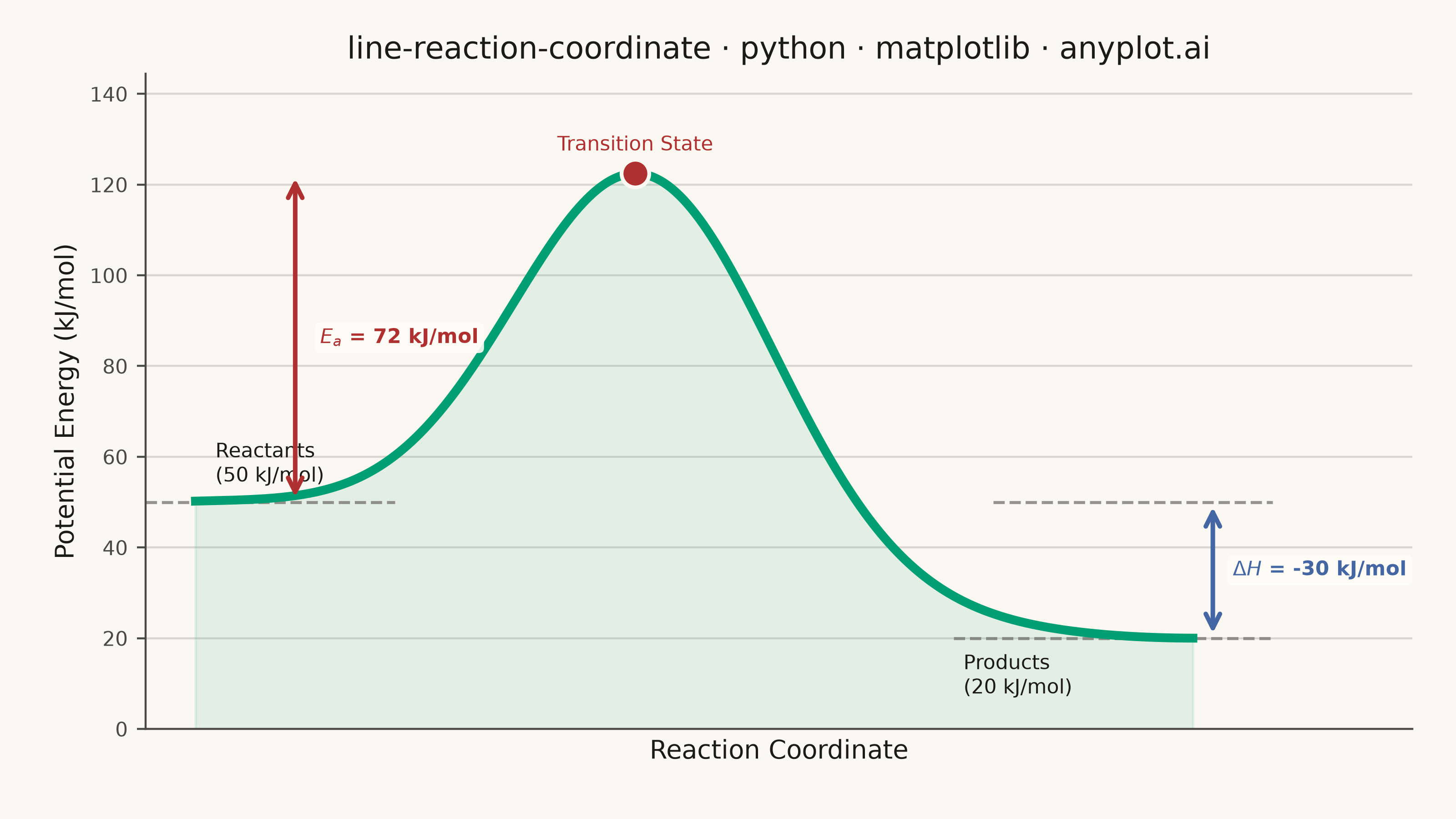
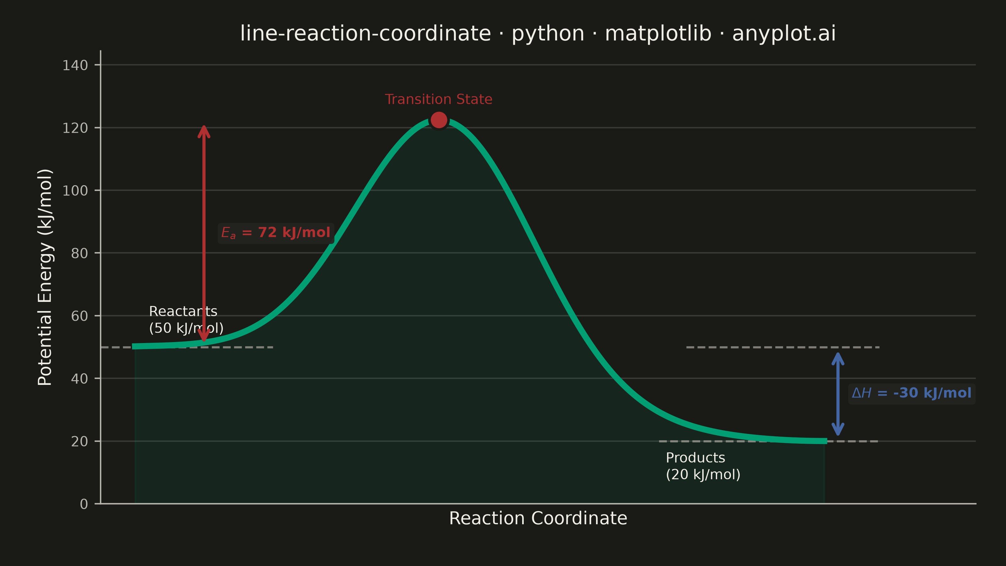
Reaction Coordinate Energy Diagram — Matplotlib

A reaction coordinate diagram plots potential energy against reaction progress, showing the energy landscape of a chemical transformation. The smooth curve traces the path from reactants through the transition state (energy maximum) to products, clearly depicting the activation energy barrier and overall enthalpy change. This fundamental chemistry visualization is essential for understanding reaction kinetics and thermodynamics.

Reaction Coordinate Energy Diagram rendered with Matplotlib

Python source (Matplotlib)

""" anyplot.ai
line-reaction-coordinate: Reaction Coordinate Energy Diagram
Library: matplotlib 3.11.0 | Python 3.13.14
Quality: 91/100 | Updated: 2026-06-24
"""

import os
import sys


# Remove the script's own directory from sys.path so that `import matplotlib`
# resolves to the installed package rather than this file (which is named matplotlib.py).
sys.path.pop(0)

import matplotlib.pyplot as plt
import numpy as np
from matplotlib.patches import FancyArrowPatch


# Theme tokens
THEME = os.getenv("ANYPLOT_THEME", "light")
PAGE_BG = "#FAF8F1" if THEME == "light" else "#1A1A17"
ELEVATED_BG = "#FFFDF6" if THEME == "light" else "#242420"
INK = "#1A1A17" if THEME == "light" else "#F0EFE8"
INK_SOFT = "#4A4A44" if THEME == "light" else "#B8B7B0"
INK_MUTED = "#6B6A63" if THEME == "light" else "#A8A79F"

# Imprint palette — position 1 for main curve; semantic red for barrier
BRAND = "#009E73"  # Imprint palette position 1 — energy pathway curve
EA_COLOR = "#AE3030"  # Imprint matte red — semantic: activation barrier (cost)
DH_COLOR = "#4467A3"  # Imprint blue — thermodynamic enthalpy change

# Data — single-step exothermic reaction
reactant_energy = 50.0
transition_energy = 120.0
product_energy = 20.0
peak_pos = 0.45

reaction_coord = np.linspace(0, 1, 500)
sigma = 0.13
baseline = reactant_energy + (product_energy - reactant_energy) * (3 * reaction_coord**2 - 2 * reaction_coord**3)
gaussian_bump = (transition_energy - (reactant_energy + product_energy) / 2) * np.exp(
    -((reaction_coord - peak_pos) ** 2) / (2 * sigma**2)
)
energy = baseline + gaussian_bump

peak_idx = np.argmax(energy)
actual_peak = energy[peak_idx]
peak_x = reaction_coord[peak_idx]

# Plot
fig, ax = plt.subplots(figsize=(8, 4.5), dpi=400, facecolor=PAGE_BG)
ax.set_facecolor(PAGE_BG)

ax.plot(reaction_coord, energy, color=BRAND, linewidth=3.5, zorder=3)
ax.fill_between(reaction_coord, 0, energy, color=BRAND, alpha=0.09, zorder=2)

# Dashed reference lines at reactant and product energy levels
ax.hlines(reactant_energy, -0.05, 0.20, colors=INK_MUTED, linestyles="--", linewidth=1.2, alpha=0.7)
ax.hlines(reactant_energy, 0.80, 1.08, colors=INK_MUTED, linestyles="--", linewidth=1.2, alpha=0.7)
ax.hlines(product_energy, 0.76, 1.08, colors=INK_MUTED, linestyles="--", linewidth=1.2, alpha=0.7)

# Transition state marker
ax.scatter([peak_x], [actual_peak], s=120, color=EA_COLOR, zorder=4, edgecolors=PAGE_BG, linewidth=1.5)

# Direct labels for reactants, products, transition state
ax.text(0.02, reactant_energy + 3, "Reactants\n(50 kJ/mol)", fontsize=8, fontweight="medium", color=INK, va="bottom")
ax.text(0.77, product_energy - 3, "Products\n(20 kJ/mol)", fontsize=8, fontweight="medium", color=INK, va="top")
ax.text(
    peak_x,
    actual_peak + 4,
    "Transition State",
    fontsize=8,
    fontweight="medium",
    color=EA_COLOR,
    va="bottom",
    ha="center",
)

# Activation energy arrow (Ea) — vertical double-headed arrow from reactant level to TS
ea_x = 0.10
arrow_ea = FancyArrowPatch(
    (ea_x, reactant_energy),
    (ea_x, actual_peak),
    arrowstyle="<->",
    mutation_scale=14,
    linewidth=1.8,
    color=EA_COLOR,
    zorder=5,
)
ax.add_patch(arrow_ea)
ea_value = actual_peak - reactant_energy
ax.text(
    ea_x + 0.025,
    (reactant_energy + actual_peak) / 2,
    f"$E_a$ = {ea_value:.0f} kJ/mol",
    fontsize=8,
    fontweight="bold",
    color=EA_COLOR,
    ha="left",
    va="center",
    bbox={"boxstyle": "round,pad=0.25", "facecolor": ELEVATED_BG, "edgecolor": "none", "alpha": 0.9},
)

# Enthalpy change arrow (ΔH) — vertical double-headed arrow on right
dh_x = 1.02
arrow_dh = FancyArrowPatch(
    (dh_x, reactant_energy),
    (dh_x, product_energy),
    arrowstyle="<->",
    mutation_scale=14,
    linewidth=1.8,
    color=DH_COLOR,
    zorder=5,
)
ax.add_patch(arrow_dh)
dh_value = product_energy - reactant_energy
ax.text(
    dh_x + 0.02,
    (reactant_energy + product_energy) / 2,
    f"$\\Delta H$ = {dh_value:.0f} kJ/mol",
    fontsize=8,
    fontweight="bold",
    color=DH_COLOR,
    ha="left",
    va="center",
    bbox={"boxstyle": "round,pad=0.25", "facecolor": ELEVATED_BG, "edgecolor": "none", "alpha": 0.9},
)

# Style
title = "line-reaction-coordinate · python · matplotlib · anyplot.ai"
ax.set_xlabel("Reaction Coordinate", fontsize=10, color=INK)
ax.set_ylabel("Potential Energy (kJ/mol)", fontsize=10, color=INK)
ax.set_title(title, fontsize=12, fontweight="medium", color=INK)
ax.tick_params(axis="both", labelsize=8, colors=INK_SOFT, labelcolor=INK_SOFT)
ax.set_xlim(-0.05, 1.22)
ax.set_ylim(0, actual_peak + 22)
ax.spines["top"].set_visible(False)
ax.spines["right"].set_visible(False)
for s in ("left", "bottom"):
    ax.spines[s].set_color(INK_SOFT)
ax.yaxis.grid(True, alpha=0.15, linewidth=0.8, color=INK)
ax.set_xticks([])

fig.subplots_adjust(left=0.10, right=0.97, top=0.91, bottom=0.11)

# Save
plt.savefig(f"plot-{THEME}.png", dpi=400, facecolor=PAGE_BG)

Part of Reaction Coordinate Energy Diagram on anyplot.ai.

Reaction Coordinate Energy Diagram — Matplotlib

Python source (Matplotlib)

Other implementations