Basic Lollipop Chart — Bokeh

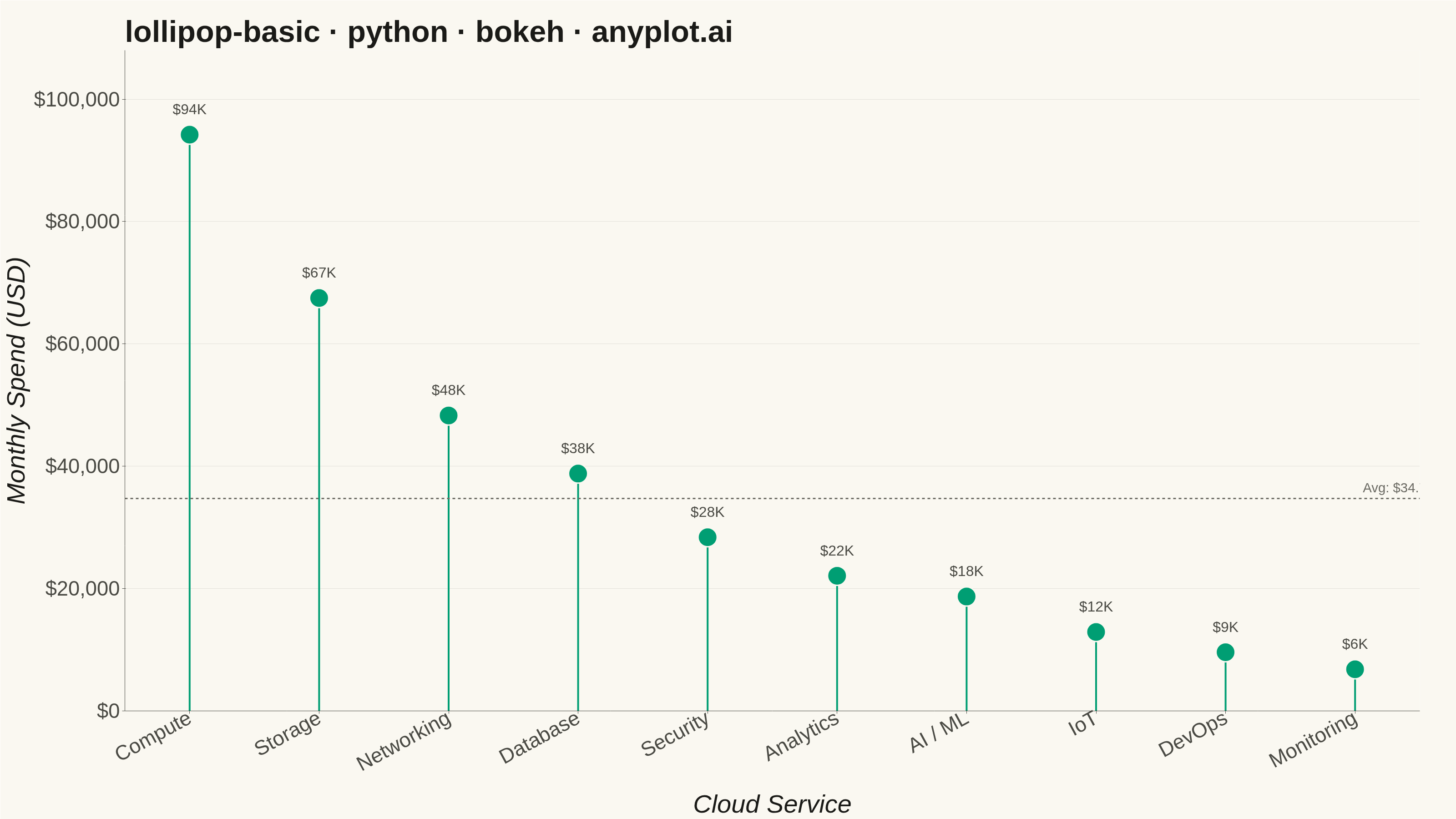
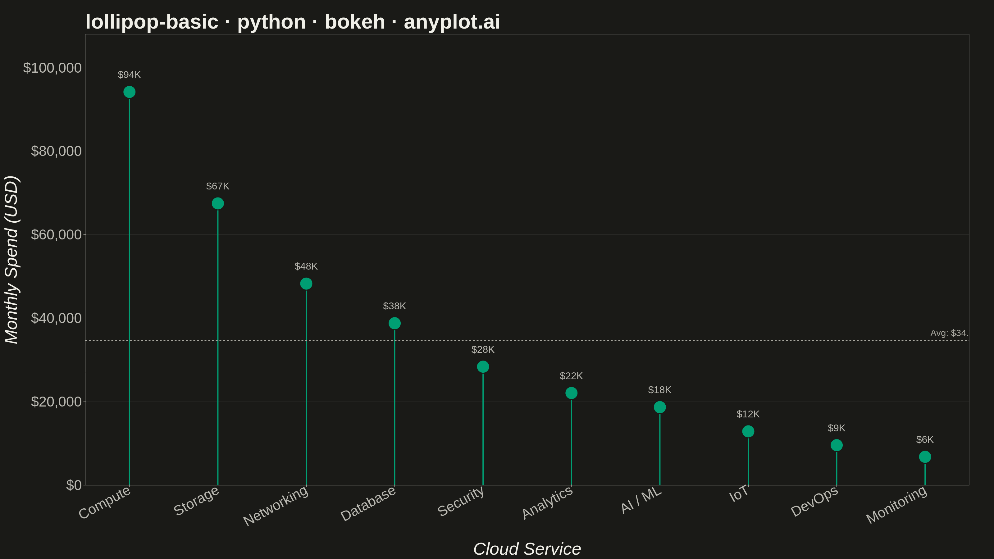
A lollipop chart displays categorical data with thin lines (stems) extending from a baseline to circular markers (dots) at each data point. It presents the same information as a bar chart but with a cleaner, more minimalist aesthetic that reduces visual clutter while maintaining clear value comparisons.
Basic Lollipop Chart rendered with Bokeh
Python source (Bokeh)

""" anyplot.ai
lollipop-basic: Basic Lollipop Chart
Library: bokeh 3.9.1 | Python 3.13.14
Quality: 91/100 | Updated: 2026-07-01
"""

import sys


# This file is named bokeh.py; without this fix Python would import itself
# instead of the installed bokeh package when run directly.
if sys.path and sys.path[0] not in ("", None):
    sys.path.append(sys.path.pop(0))

import io
import os
import time
from pathlib import Path

from bokeh.io import output_file, save
from bokeh.models import ColumnDataSource, Label, NumeralTickFormatter, Range1d, Span
from bokeh.plotting import figure
from PIL import Image
from selenium import webdriver
from selenium.webdriver.chrome.options import Options


# Imprint palette + theme tokens
THEME = os.getenv("ANYPLOT_THEME", "light")
PAGE_BG = "#FAF8F1" if THEME == "light" else "#1A1A17"
INK = "#1A1A17" if THEME == "light" else "#F0EFE8"
INK_SOFT = "#4A4A44" if THEME == "light" else "#B8B7B0"
INK_MUTED = "#6B6A63" if THEME == "light" else "#A8A79F"
BRAND = "#009E73"  # Imprint palette position 1 — always first series

# Data — monthly cloud infrastructure spend by service category (sorted descending)
categories = [
    "Compute",
    "Storage",
    "Networking",
    "Database",
    "Security",
    "Analytics",
    "AI / ML",
    "IoT",
    "DevOps",
    "Monitoring",
]
values = [94200, 67500, 48300, 38800, 28400, 22100, 18700, 12900, 9600, 6800]
avg_spend = sum(values) / len(values)

labels = [f"${v // 1000}K" for v in values]

source = ColumnDataSource(
    data={
        "categories": categories,
        "values": values,
        "zeros": [0] * len(values),
        "labels": labels,
        "label_y": [v + 2800 for v in values],
    }
)

# Figure
p = figure(
    width=3200,
    height=1800,
    x_range=categories,
    y_range=Range1d(0, 108000),
    title="lollipop-basic · python · bokeh · anyplot.ai",
    x_axis_label="Cloud Service",
    y_axis_label="Monthly Spend (USD)",
    toolbar_location=None,
    min_border_bottom=160,
    min_border_left=180,
    min_border_top=110,
    min_border_right=80,
)

# Average reference line + label
p.add_layout(Span(location=avg_spend, dimension="width", line_color=INK_MUTED, line_width=3, line_dash="dashed"))
p.add_layout(
    Label(
        x=2880,
        y=avg_spend,  # screen x from plot-frame left; plot area = 3200-180-80=2940px wide
        x_units="screen",
        text=f"Avg: ${avg_spend / 1000:.1f}K",
        text_font_size="22pt",
        text_color=INK_MUTED,
        text_align="right",
        text_baseline="bottom",
        y_offset=8,
    )
)

# Stems
p.segment(x0="categories", y0="zeros", x1="categories", y1="values", source=source, line_width=4, color=BRAND)

# Markers
p.scatter(x="categories", y="values", source=source, size=42, color=BRAND, line_color=PAGE_BG, line_width=3)

# Value labels above each marker
p.text(
    x="categories",
    y="label_y",
    text="labels",
    source=source,
    text_font_size="24pt",
    text_align="center",
    text_baseline="bottom",
    text_color=INK_SOFT,
)

# Title
p.title.text_font_size = "50pt"
p.title.text_color = INK
p.title.text_font_style = "bold"

# Axis label sizes
p.xaxis.axis_label_text_font_size = "42pt"
p.yaxis.axis_label_text_font_size = "42pt"
p.xaxis.major_label_text_font_size = "34pt"
p.yaxis.major_label_text_font_size = "34pt"

# Axis label colors
p.xaxis.axis_label_text_color = INK
p.yaxis.axis_label_text_color = INK
p.xaxis.major_label_text_color = INK_SOFT
p.yaxis.major_label_text_color = INK_SOFT

# Axis line and tick colors
p.xaxis.axis_line_color = INK_SOFT
p.yaxis.axis_line_color = INK_SOFT
p.xaxis.major_tick_line_color = INK_SOFT
p.yaxis.major_tick_line_color = INK_SOFT
p.xaxis.minor_tick_line_color = None
p.yaxis.minor_tick_line_color = None
p.xaxis.major_label_orientation = 0.5

# Grid — y-axis only, subtle
p.xgrid.grid_line_color = None
p.ygrid.grid_line_color = INK
p.ygrid.grid_line_alpha = 0.10

# Background and chrome
p.background_fill_color = PAGE_BG
p.border_fill_color = PAGE_BG
p.outline_line_color = None  # L-spine only: x/y axis_line_color handle bottom+left

# Y-axis tick format
p.yaxis.formatter = NumeralTickFormatter(format="$0,0")

# Save HTML (interactive catalog artifact)
output_file(f"plot-{THEME}.html")
save(p)

# Screenshot with headless Chrome — Selenium 4 / Selenium Manager resolves the driver.
# Chrome's headless viewport is ~143px shorter than --window-size due to internal
# overhead; use an oversized window then crop to the exact canvas target.
W, H = 3200, 1800
CHROME_H = H + 200
opts = Options()
for arg in (
    "--headless=new",
    "--no-sandbox",
    "--disable-dev-shm-usage",
    "--disable-gpu",
    f"--window-size={W},{CHROME_H}",
    "--hide-scrollbars",
):
    opts.add_argument(arg)
driver = webdriver.Chrome(options=opts)
driver.set_window_size(W, CHROME_H)
driver.get(f"file://{Path(f'plot-{THEME}.html').resolve()}")
time.sleep(3)
# The bokeh figure starts at (0, 0); crop screenshot to exact canvas dimensions
Image.open(io.BytesIO(driver.get_screenshot_as_png())).crop((0, 0, W, H)).save(f"plot-{THEME}.png")
driver.quit()
Part of Basic Lollipop Chart on anyplot.ai.
Basic Lollipop Chart — Bokeh

Python source (Bokeh)

Other implementations
