The same plot in 14 other libraries — Python: Altair, Bokeh, lets-plot, Matplotlib, Plotly, plotnine, Pygal, Seaborn; R: ggplot2; JavaScript: Chart.js, D3.js, Apache ECharts, Highcharts, MUI X Charts. Compare all 15 side by side: Weighted Network Graph with Edge Thickness in Python, R, Julia and JavaScript.
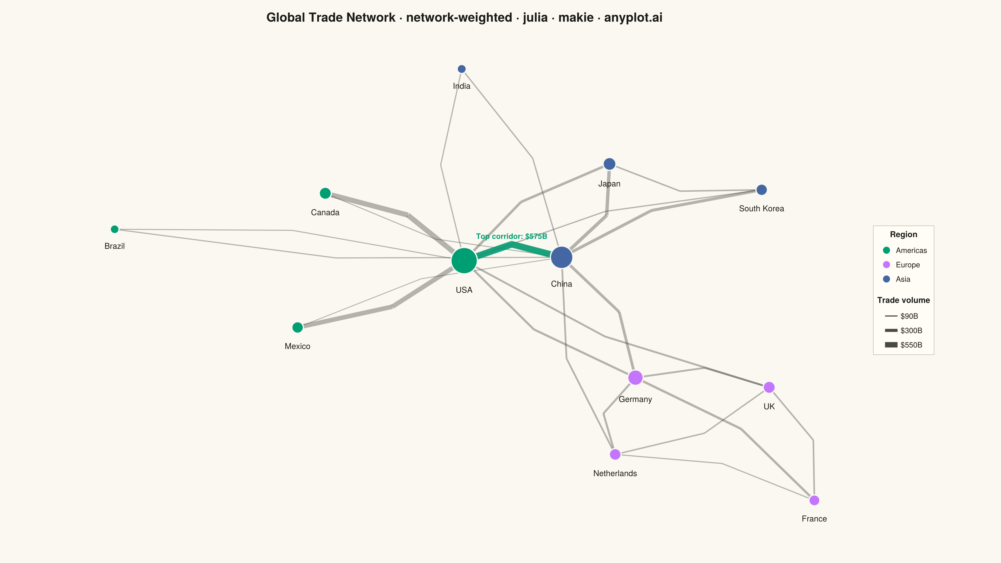
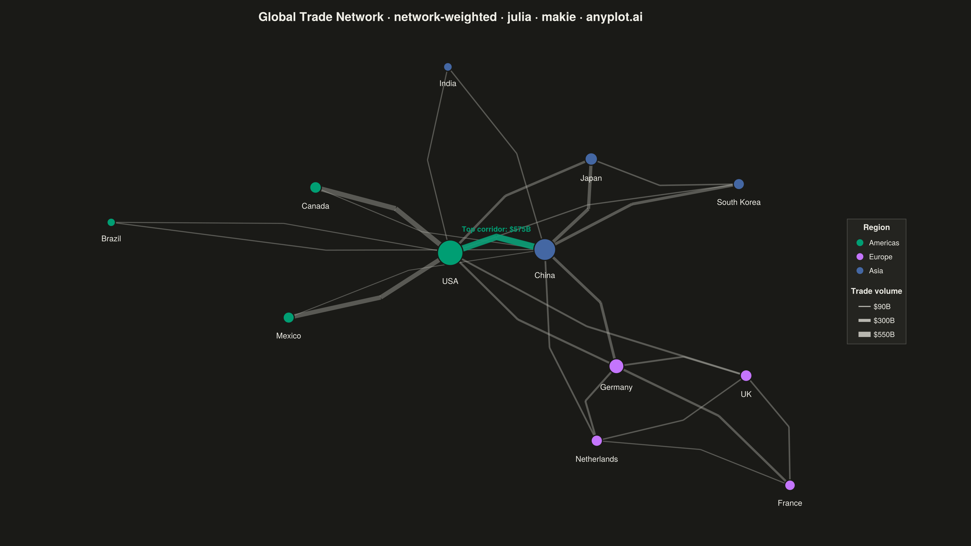
A weighted network graph displays relationships between entities using edge thickness to represent connection strength or weight. Unlike basic network graphs where edges are uniform, the varying line widths immediately communicate the relative importance of each relationship. This visualization makes it easy to identify strong vs weak connections, central hubs with many heavy links, and structural patterns in weighted relational data.
# anyplot.ai
# network-weighted: Weighted Network Graph with Edge Thickness
# Library: makie 0.21.9 | Julia 1.11.9
# Quality: 94/100 | Created: 2026-09-02

using CairoMakie
using Colors
using Random
using Statistics

Random.seed!(42)

# --- Theme tokens -----------------------------------------------------------
const THEME       = get(ENV, "ANYPLOT_THEME", "light")
const PAGE_BG     = THEME == "light" ? colorant"#FAF8F1" : colorant"#1A1A17"
const ELEVATED_BG = THEME == "light" ? colorant"#FFFDF6" : colorant"#242420"
const INK         = THEME == "light" ? colorant"#1A1A17" : colorant"#F0EFE8"
const INK_SOFT    = THEME == "light" ? colorant"#4A4A44" : colorant"#B8B7B0"

const IMPRINT_PALETTE = [
    colorant"#009E73",  # 1 — Americas
    colorant"#C475FD",  # 2 — Europe
    colorant"#4467A3",  # 3 — Asia
]

# --- Data: bilateral trade network, annual volume in billions USD ----------
countries = [
    "USA", "China", "Germany", "Japan", "UK", "France",
    "India", "Brazil", "South Korea", "Canada", "Mexico", "Netherlands",
]
region = [1, 3, 2, 3, 2, 2, 3, 1, 3, 1, 1, 2]
region_names = ["Americas", "Europe", "Asia"]
n = length(countries)

# (source, target, weight) — weight is annual trade volume in $B, scaled to
# realistic bilateral-trade magnitudes while preserving the relative ranking
# (China/Canada/Mexico as USA's top partners)
edges = [
    (1, 2, 575), (1, 10, 520), (1, 11, 460), (1, 3, 200), (1, 4, 240), (1, 5, 175),
    (2, 3, 265), (2, 4, 330), (2, 9, 285), (2, 12, 155),
    (3, 6, 220), (3, 12, 185), (3, 5, 165),
    (6, 5, 140), (5, 12, 120), (4, 9, 130),
    (7, 2, 110), (7, 1, 95),
    (8, 1, 80), (8, 2, 90),
    (11, 2, 65), (10, 2, 75),
    (12, 6, 90), (9, 1, 105),
]
weights = [w for (_, _, w) in edges]
min_weight, max_weight = extrema(weights)
mean_weight = mean(weights)

weighted_degree = zeros(Int, n)
for (a, b, w) in edges
    weighted_degree[a] += w
    weighted_degree[b] += w
end

# --- Force-directed layout, weight-scaled attraction (hand-rolled
#     Fruchterman-Reingold — no NetworkLayout.jl, which is not installed
#     in the CI runtime). Heavier edges pull their endpoints closer. --------
pos_x = randn(n) .* 3.0
pos_y = randn(n) .* 3.0
k = sqrt(180.0 / n)

for iter in 0:299
    t_step = max(1.0 * 0.97^iter, 0.005)
    dx = zeros(n)
    dy = zeros(n)

    for i in 1:n, j in 1:n
        if i != j
            δx = pos_x[i] - pos_x[j]
            δy = pos_y[i] - pos_y[j]
            d  = max(sqrt(δx^2 + δy^2), 1e-4)
            f  = k^2 / d
            dx[i] += δx / d * f
            dy[i] += δy / d * f
        end
    end

    for (a, b, w) in edges
        δx = pos_x[a] - pos_x[b]
        δy = pos_y[a] - pos_y[b]
        d  = max(sqrt(δx^2 + δy^2), 1e-4)
        f  = (w / mean_weight) * d^2 / k
        dx[a] -= δx / d * f
        dy[a] -= δy / d * f
        dx[b] += δx / d * f
        dy[b] += δy / d * f
    end

    for i in 1:n
        disp = sqrt(dx[i]^2 + dy[i]^2)
        if disp > 0
            pos_x[i] += dx[i] / disp * min(disp, t_step)
            pos_y[i] += dy[i] / disp * min(disp, t_step)
        end
    end
end

pos_x = 0.06 .+ 0.88 .* (pos_x .- minimum(pos_x)) ./ (maximum(pos_x) - minimum(pos_x))
pos_y = 0.10 .+ 0.82 .* (pos_y .- minimum(pos_y)) ./ (maximum(pos_y) - minimum(pos_y))

node_colors = [IMPRINT_PALETTE[region[i]] for i in 1:n]
node_sizes  = 20.0 .+ 40.0 .* (weighted_degree .- minimum(weighted_degree)) ./
              (maximum(weighted_degree) - minimum(weighted_degree))

# --- Plot ---------------------------------------------------------------
title_text = "Global Trade Network · network-weighted · julia · makie · anyplot.ai"
title_size = length(title_text) > 67 ? round(Int, 20 * 67 / length(title_text)) : 20

fig = Figure(
    size            = (1600, 900),
    fontsize        = 14,
    backgroundcolor = PAGE_BG,
)

ax = Axis(
    fig[1, 1];
    title              = title_text,
    titlesize          = title_size,
    titlecolor         = INK,
    backgroundcolor    = PAGE_BG,
    topspinevisible    = false,
    rightspinevisible  = false,
    leftspinevisible   = false,
    bottomspinevisible = false,
    xgridvisible       = false,
    ygridvisible       = false,
    xticksvisible      = false,
    yticksvisible      = false,
    xticklabelsvisible = false,
    yticklabelsvisible = false,
)

limits!(ax, 0, 1, 0, 1)

# Edges — linewidth encodes trade volume, the spec's primary signal. Each
# edge is a 2-segment polyline bowed through a perpendicular-offset midpoint
# (sign alternating by index) so near-parallel edges converging on the same
# hub node stay visually separable instead of overlapping — still a single
# batched linesegments! call.
edge_points = Vector{Point2f}(undef, 4 * length(edges))
edge_widths = Vector{Float32}(undef, 4 * length(edges))
edge_mid    = Vector{Point2f}(undef, length(edges))
top_idx     = argmax(weights)
for (idx, (a, b, w)) in enumerate(edges)
    p1 = Point2f(pos_x[a], pos_y[a])
    p2 = Point2f(pos_x[b], pos_y[b])
    edx, edy = pos_x[b] - pos_x[a], pos_y[b] - pos_y[a]
    ed = max(sqrt(edx^2 + edy^2), 1e-4)
    perp_x, perp_y = -edy / ed, edx / ed
    curve_sign = isodd(idx) ? 1.0 : -1.0
    mx, my = (pos_x[a] + pos_x[b]) / 2, (pos_y[a] + pos_y[b]) / 2
    mid = Point2f(mx + perp_x * 0.028 * curve_sign, my + perp_y * 0.028 * curve_sign)
    edge_mid[idx] = mid

    width = 1.4 + (w - min_weight) / (max_weight - min_weight) * (9.0 - 1.4)
    edge_points[4idx - 3] = p1
    edge_points[4idx - 2] = mid
    edge_points[4idx - 1] = mid
    edge_points[4idx]     = p2
    edge_widths[4idx - 3] = width
    edge_widths[4idx - 2] = width
    edge_widths[4idx - 1] = width
    edge_widths[4idx]     = width
end
linesegments!(ax, edge_points; color = (INK_SOFT, 0.4), linewidth = edge_widths)

# Highlight the single strongest trade corridor as a sharper storytelling focal point
top_a, top_b, top_w = edges[top_idx]
top_width = 1.4 + (top_w - min_weight) / (max_weight - min_weight) * (9.0 - 1.4)
lines!(
    ax,
    [Point2f(pos_x[top_a], pos_y[top_a]), edge_mid[top_idx], Point2f(pos_x[top_b], pos_y[top_b])];
    color     = (IMPRINT_PALETTE[1], 0.85),
    linewidth = top_width + 1.5,
)
text!(
    ax, [edge_mid[top_idx][1]], [edge_mid[top_idx][2]];
    text     = ["Top corridor: \$$(top_w)B"],
    fontsize = 12,
    font     = :bold,
    color    = IMPRINT_PALETTE[1],
    align    = (:center, :bottom),
    offset   = (0.0f0, 6.0f0),
)

# Nodes — size encodes weighted degree (total trade volume), color encodes region
scatter!(
    ax, pos_x, pos_y;
    color       = node_colors,
    markersize  = node_sizes,
    strokewidth = 2.0,
    strokecolor = PAGE_BG,
)

text!(
    ax, pos_x, pos_y;
    text     = countries,
    align    = (:center, :top),
    fontsize = 13,
    color    = INK,
    offset   = [(0.0f0, -(node_sizes[i] / 2 + 9)) for i in 1:n],
)

# Legend — region color + trade-volume line-width scale
region_elems = [
    MarkerElement(color = IMPRINT_PALETTE[i], marker = :circle, markersize = 16, strokewidth = 0)
    for i in 1:3
]
weight_samples = [90, 300, 550]
weight_elems = [
    LineElement(color = INK_SOFT, linewidth = 1.4 + (w - min_weight) / (max_weight - min_weight) * (9.0 - 1.4))
    for w in weight_samples
]
weight_labels = ["\$$(w)B" for w in weight_samples]

Legend(
    fig[1, 2],
    [region_elems, weight_elems],
    [region_names, weight_labels],
    ["Region", "Trade volume"];
    titlesize       = 13,
    titlecolor      = INK,
    labelsize       = 12,
    labelcolor      = INK,
    framevisible    = true,
    framecolor      = (INK_SOFT, 0.3),
    backgroundcolor = ELEVATED_BG,
)

colsize!(fig.layout, 1, Relative(0.82))

# Save
save("plot-$(THEME).png", fig; px_per_unit = 2)
Runnable source as JSON, for any HTTP client: https://api.anyplot.ai/specs/network-weighted/makie/code. Any spec id and library id listed in llms-full.txt fit the same URL shape; every URL below is complete and callable.
{
  "spec_id": "network-weighted",
  "language": "julia",
  "library": "makie",
  "page": "https://anyplot.ai/network-weighted/julia/makie",
  "hub": "https://anyplot.ai/network-weighted",
  "code_json": "https://api.anyplot.ai/specs/network-weighted/makie/code",
  "spec_json": "https://api.anyplot.ai/specs/network-weighted",
  "render_light_png": "https://storage.googleapis.com/anyplot-images/plots/network-weighted/julia/makie/plot-light.png",
  "render_dark_png": "https://storage.googleapis.com/anyplot-images/plots/network-weighted/julia/makie/plot-dark.png",
  "quality_score": 94.0,
  "license": "MIT",
  "guide": "https://anyplot.ai/llms.txt"
}
Part of Weighted Network Graph with Edge Thickness on anyplot.ai.