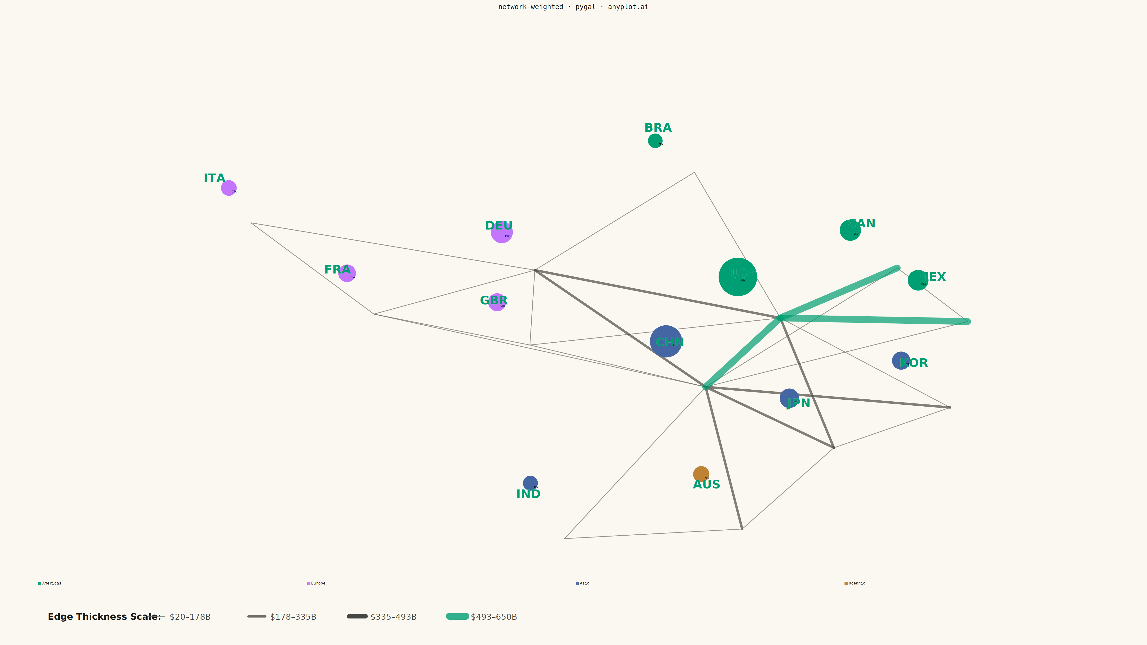
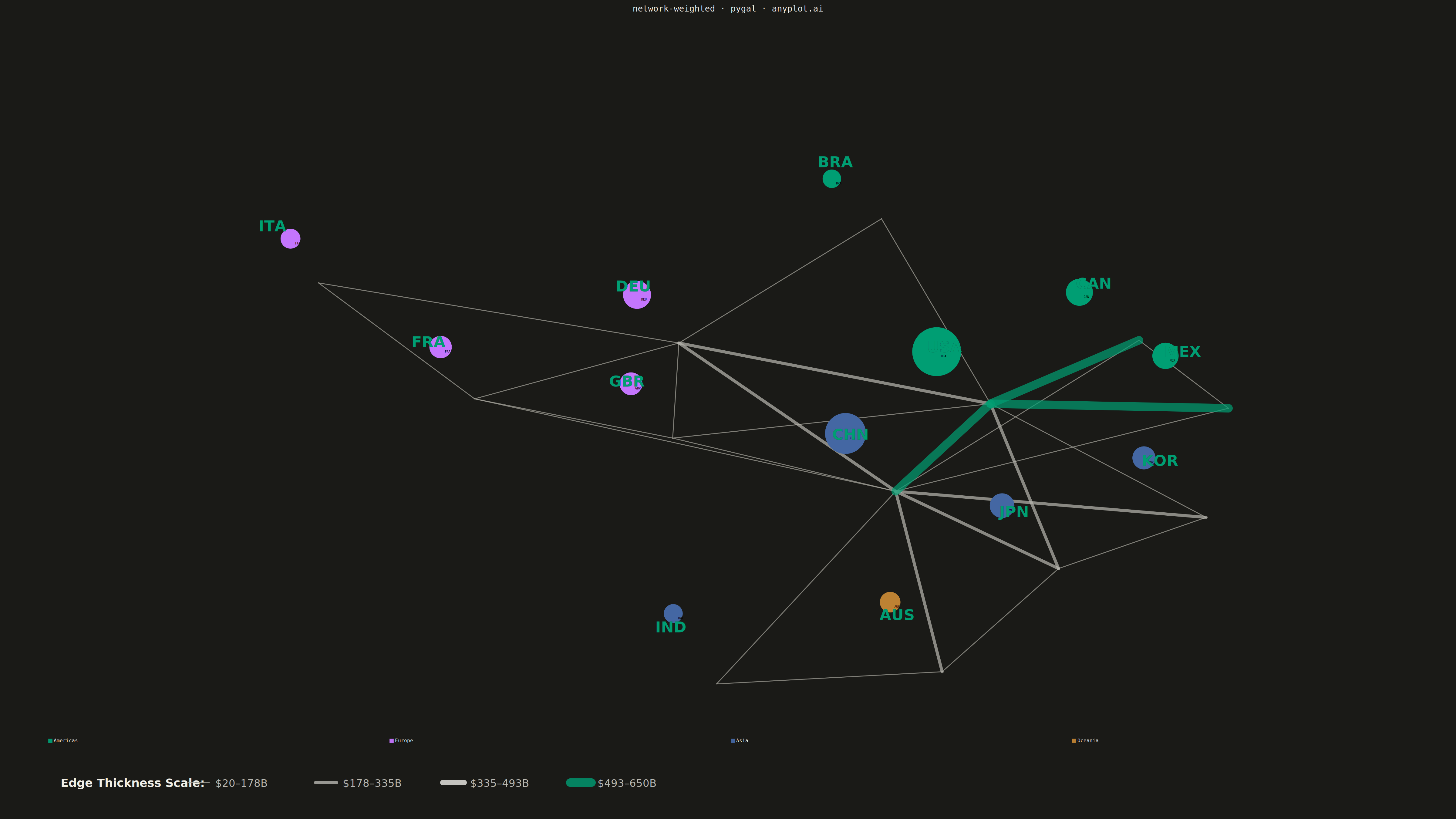
A weighted network graph displays relationships between entities using edge thickness to represent connection strength or weight. Unlike basic network graphs where edges are uniform, the varying line widths immediately communicate the relative importance of each relationship. This visualization makes it easy to identify strong vs weak connections, central hubs with many heavy links, and structural patterns in weighted relational data.
""" anyplot.ai
network-weighted: Weighted Network Graph with Edge Thickness
Library: pygal 3.1.0 | Python 3.13.13
Quality: 92/100 | Updated: 2026-05-17
"""

import os
import re
import sys
from pathlib import Path


# Work around filename/module name conflict
script_dir = Path(__file__).parent
while str(script_dir) in sys.path:
    sys.path.remove(str(script_dir))

import cairosvg
import numpy as np
import pygal
from pygal.style import Style


# Theme tokens
THEME = os.getenv("ANYPLOT_THEME", "light")
PAGE_BG = "#FAF8F1" if THEME == "light" else "#1A1A17"
ELEVATED_BG = "#FFFDF6" if THEME == "light" else "#242420"
INK = "#1A1A17" if THEME == "light" else "#F0EFE8"
INK_SOFT = "#4A4A44" if THEME == "light" else "#B8B7B0"
INK_MUTED = "#6B6A63" if THEME == "light" else "#A8A79F"

# Okabe-Ito palette
IMPRINT = ("#009E73", "#C475FD", "#4467A3", "#BD8233", "#AE3030", "#2ABCCD", "#954477")

# Data: Trade network between countries (billions USD)
np.random.seed(42)
nodes = {
    "USA": {"group": 0},
    "CAN": {"group": 0},
    "MEX": {"group": 0},
    "BRA": {"group": 0},
    "DEU": {"group": 1},
    "FRA": {"group": 1},
    "GBR": {"group": 1},
    "ITA": {"group": 1},
    "CHN": {"group": 2},
    "JPN": {"group": 2},
    "KOR": {"group": 2},
    "IND": {"group": 2},
    "AUS": {"group": 3},
}

# Define edges with trade volume weights (billions USD)
edges = [
    ("USA", "CAN", 650),
    ("USA", "MEX", 580),
    ("USA", "CHN", 520),
    ("USA", "JPN", 180),
    ("USA", "DEU", 200),
    ("USA", "GBR", 130),
    ("USA", "KOR", 140),
    ("USA", "BRA", 80),
    ("CAN", "CHN", 75),
    ("CAN", "MEX", 40),
    ("MEX", "CHN", 90),
    ("DEU", "FRA", 170),
    ("DEU", "GBR", 120),
    ("DEU", "ITA", 130),
    ("DEU", "CHN", 200),
    ("FRA", "GBR", 90),
    ("FRA", "ITA", 80),
    ("FRA", "CHN", 65),
    ("GBR", "CHN", 95),
    ("CHN", "JPN", 280),
    ("CHN", "KOR", 250),
    ("CHN", "AUS", 180),
    ("CHN", "IND", 100),
    ("JPN", "KOR", 70),
    ("JPN", "AUS", 55),
    ("IND", "AUS", 30),
    ("BRA", "DEU", 20),
]

# Force-directed layout computation
node_list = list(nodes.keys())
n = len(node_list)
node_idx = {name: i for i, name in enumerate(node_list)}

# Initialize positions randomly
pos = np.random.rand(n, 2) * 2 - 1

k = 1.5 / np.sqrt(n)  # Optimal distance
t = 0.5  # Temperature (step size)

for _ in range(300):
    disp = np.zeros((n, 2))

    # Repulsive forces between all pairs
    for i in range(n):
        for j in range(i + 1, n):
            delta = pos[i] - pos[j]
            dist = max(np.linalg.norm(delta), 0.01)
            force = k * k / dist * 1.5
            direction = delta / dist
            disp[i] += direction * force
            disp[j] -= direction * force

    # Attractive forces along edges (weighted)
    for src, tgt, weight in edges:
        i, j = node_idx[src], node_idx[tgt]
        delta = pos[i] - pos[j]
        dist = max(np.linalg.norm(delta), 0.01)
        force = dist * dist / k * (0.8 + weight / 400)
        direction = delta / dist
        disp[i] -= direction * force
        disp[j] += direction * force

    # Apply displacement with temperature limiting
    for i in range(n):
        disp_norm = max(np.linalg.norm(disp[i]), 0.01)
        pos[i] += disp[i] / disp_norm * min(disp_norm, t)

    t *= 0.97

# Normalize positions to [2, 10] for pygal
pos_min = pos.min(axis=0)
pos_max = pos.max(axis=0)
pos = (pos - pos_min) / (pos_max - pos_min + 1e-6) * 8 + 2
positions = {name: pos[node_idx[name]] for name in node_list}

# Compute weighted degree for node sizing
weighted_degree = dict.fromkeys(nodes, 0)
for src, tgt, weight in edges:
    weighted_degree[src] += weight
    weighted_degree[tgt] += weight

max_degree = max(weighted_degree.values())
min_degree = min(weighted_degree.values())

# Bin edges by weight for visual thickness representation
edge_weights = [w for _, _, w in edges]
min_weight = min(edge_weights)
max_weight = max(edge_weights)
weight_range = max_weight - min_weight

# Create 4 weight bins for edge thickness visualization
edge_bins = {"low": [], "medium": [], "high": [], "very_high": []}

for src, tgt, weight in edges:
    norm_weight = (weight - min_weight) / weight_range if weight_range > 0 else 0.5
    if norm_weight < 0.25:
        edge_bins["low"].append((src, tgt, weight))
    elif norm_weight < 0.5:
        edge_bins["medium"].append((src, tgt, weight))
    elif norm_weight < 0.75:
        edge_bins["high"].append((src, tgt, weight))
    else:
        edge_bins["very_high"].append((src, tgt, weight))

# Edge thickness and color mapping based on weight
edge_styles = {
    "low": {"stroke": INK_MUTED, "stroke_width": 3},
    "medium": {"stroke": INK_SOFT, "stroke_width": 10},
    "high": {"stroke": INK, "stroke_width": 18},
    "very_high": {"stroke": IMPRINT[0], "stroke_width": 28},
}

# Custom style for pygal chart
custom_style = Style(
    background=PAGE_BG,
    plot_background=PAGE_BG,
    foreground=INK,
    foreground_strong=INK,
    foreground_subtle=INK_MUTED,
    colors=IMPRINT,
    title_font_size=28,
    label_font_size=22,
    major_label_font_size=18,
    legend_font_size=16,
    value_font_size=14,
    stroke_width=2,
    opacity=0.95,
)

# Create pygal XY chart for nodes
chart = pygal.XY(
    width=4800,
    height=2700,
    style=custom_style,
    title="network-weighted · pygal · anyplot.ai",
    show_legend=True,
    show_x_guides=False,
    show_y_guides=False,
    show_x_labels=False,
    show_y_labels=False,
    stroke=False,
    legend_at_bottom=True,
    legend_at_bottom_columns=4,
    range=(0, 12),
    xrange=(0, 12),
    print_labels=True,
    print_values=False,
    margin_bottom=250,
    margin_top=150,
    margin_left=150,
    margin_right=150,
)

# Group nodes by region and add to chart with varying dot sizes
regions = [[], [], [], []]
region_names = ["Americas", "Europe", "Asia", "Oceania"]
for name, data in nodes.items():
    regions[data["group"]].append(name)

for group_idx, region_nodes in enumerate(regions):
    node_points = []
    for name in region_nodes:
        x, y = positions[name]
        degree_norm = (
            (weighted_degree[name] - min_degree) / (max_degree - min_degree) if max_degree > min_degree else 0.5
        )
        dot_size = 30 + degree_norm * 50
        node_points.append({"value": (x, y), "label": name, "node": {"r": dot_size}})
    chart.add(region_names[group_idx], node_points, dots_size=50)

# Render chart to get SVG string
svg_content = chart.render().decode("utf-8")

# Post-process SVG to add edges with varying thickness before nodes
series_match = re.search(r"(<g class=\"series)", svg_content)
if series_match:
    insert_pos = series_match.start()
else:
    insert_pos = svg_content.rfind("</svg>")

# Calculate SVG coordinate transformation
svg_margin = {"top": 150, "right": 150, "bottom": 250, "left": 150}
svg_width = 4800
svg_height = 2700
plot_width = svg_width - svg_margin["left"] - svg_margin["right"]
plot_height = svg_height - svg_margin["top"] - svg_margin["bottom"]

# Build edge SVG elements
edge_svg_parts = ['<g class="edges">']

for weight_cat in ["low", "medium", "high", "very_high"]:
    style = edge_styles[weight_cat]
    for src, tgt, _weight in edge_bins[weight_cat]:
        x1_data, y1_data = positions[src]
        x2_data, y2_data = positions[tgt]

        x1 = svg_margin["left"] + (x1_data / 12) * plot_width
        y1 = svg_margin["top"] + (1 - y1_data / 12) * plot_height
        x2 = svg_margin["left"] + (x2_data / 12) * plot_width
        y2 = svg_margin["top"] + (1 - y2_data / 12) * plot_height

        edge_svg_parts.append(
            f'<line x1="{x1:.1f}" y1="{y1:.1f}" x2="{x2:.1f}" y2="{y2:.1f}" '
            f'stroke="{style["stroke"]}" stroke-width="{style["stroke_width"]}" '
            f'stroke-linecap="round" opacity="0.7"/>'
        )

edge_svg_parts.append("</g>")
edge_svg = "\n".join(edge_svg_parts)

# Insert edges into SVG
svg_content = svg_content[:insert_pos] + edge_svg + "\n" + svg_content[insert_pos:]

# Add node labels (country codes) on top of nodes
label_svg_parts = ['<g class="node-labels">']
for name in nodes.keys():
    x_data, y_data = positions[name]
    x = svg_margin["left"] + (x_data / 12) * plot_width
    y = svg_margin["top"] + (1 - y_data / 12) * plot_height

    # White stroke for contrast
    label_svg_parts.append(
        f'<text x="{x:.1f}" y="{y + 18:.1f}" text-anchor="middle" '
        f'font-family="system-ui, sans-serif" font-size="50" font-weight="bold" '
        f'fill="{PAGE_BG}" stroke="{PAGE_BG}" stroke-width="10">{name}</text>'
    )
    # Main text in brand color
    label_svg_parts.append(
        f'<text x="{x:.1f}" y="{y + 18:.1f}" text-anchor="middle" '
        f'font-family="system-ui, sans-serif" font-size="50" font-weight="bold" '
        f'fill="{IMPRINT[0]}">{name}</text>'
    )

label_svg_parts.append("</g>")
label_svg = "\n".join(label_svg_parts)

# Insert labels before closing </svg>
svg_content = svg_content.replace("</svg>", label_svg + "\n</svg>")

# Add edge weight legend
legend_y = 2700 - 120
legend_x_start = 200
legend_items = [
    ("$20–178B", edge_styles["low"]),
    ("$178–335B", edge_styles["medium"]),
    ("$335–493B", edge_styles["high"]),
    ("$493–650B", edge_styles["very_high"]),
]

edge_legend_parts = ['<g class="edge-legend">']
edge_legend_parts.append(
    f'<text x="{legend_x_start}" y="{legend_y + 14}" '
    f'font-family="system-ui, sans-serif" font-size="38" font-weight="bold" '
    f'fill="{INK}">Edge Thickness Scale:</text>'
)
legend_x = legend_x_start + 420
for label, style in legend_items:
    edge_legend_parts.append(
        f'<line x1="{legend_x}" y1="{legend_y}" x2="{legend_x + 70}" y2="{legend_y}" '
        f'stroke="{style["stroke"]}" stroke-width="{style["stroke_width"]}" '
        f'stroke-linecap="round" opacity="0.8"/>'
    )
    edge_legend_parts.append(
        f'<text x="{legend_x + 90}" y="{legend_y + 14}" '
        f'font-family="system-ui, sans-serif" font-size="34" fill="{INK_SOFT}">{label}</text>'
    )
    legend_x += 420

edge_legend_parts.append("</g>")
edge_legend_svg = "\n".join(edge_legend_parts)

# Insert edge legend before closing </svg>
svg_content = svg_content.replace("</svg>", edge_legend_svg + "\n</svg>")

# Convert modified SVG to PNG using cairosvg
cairosvg.svg2png(bytestring=svg_content.encode("utf-8"), write_to=f"plot-{THEME}.png")

# Save interactive HTML version
with open(f"plot-{THEME}.html", "w") as f:
    f.write(
        f"""<!DOCTYPE html>
<html>
<head>
    <meta charset="utf-8">
    <title>network-weighted · pygal · anyplot.ai</title>
    <style>
        body {{
            margin: 0;
            padding: 20px;
            background-color: {PAGE_BG};
            font-family: system-ui, sans-serif;
        }}
        .container {{
            max-width: 4800px;
            margin: 0 auto;
        }}
        h1 {{
            color: {INK};
            text-align: center;
            margin-bottom: 30px;
        }}
        .chart-container {{
            display: flex;
            justify-content: center;
        }}
        img {{
            max-width: 100%;
            height: auto;
            border-radius: 8px;
            box-shadow: 0 4px 12px rgba(0, 0, 0, 0.1);
        }}
        .info {{
            color: {INK_SOFT};
            text-align: center;
            margin-top: 20px;
            font-size: 16px;
        }}
    </style>
</head>
<body>
    <div class="container">
        <h1>network-weighted · pygal · anyplot.ai</h1>
        <div class="chart-container">
            <img src="plot-{THEME}.png" alt="Network graph with weighted edges">
        </div>
        <div class="info">
            <p>Trade network visualization showing relationships between countries.</p>
            <p>Edge thickness represents bilateral trade volume (billions USD).</p>
            <p>Node size indicates total weighted degree (sum of connected edge weights).</p>
        </div>
    </div>
</body>
</html>"""
    )
Runnable source as JSON, for any HTTP client: https://api.anyplot.ai/specs/network-weighted/pygal/code. Any spec id and library id listed in llms-full.txt fit the same URL shape; every URL below is complete and callable.
{
  "spec_id": "network-weighted",
  "language": "python",
  "library": "pygal",
  "page": "https://anyplot.ai/network-weighted/python/pygal",
  "hub": "https://anyplot.ai/network-weighted",
  "code_json": "https://api.anyplot.ai/specs/network-weighted/pygal/code",
  "spec_json": "https://api.anyplot.ai/specs/network-weighted",
  "render_light_png": "https://storage.googleapis.com/anyplot-images/plots/network-weighted/python/pygal/plot-light.png",
  "render_dark_png": "https://storage.googleapis.com/anyplot-images/plots/network-weighted/python/pygal/plot-dark.png",
  "interactive_light_html": "https://storage.googleapis.com/anyplot-images/plots/network-weighted/python/pygal/plot-light.html",
  "interactive_dark_html": "https://storage.googleapis.com/anyplot-images/plots/network-weighted/python/pygal/plot-dark.html",
  "quality_score": 92.0,
  "license": "MIT",
  "guide": "https://anyplot.ai/llms.txt"
}
Part of Weighted Network Graph with Edge Thickness on anyplot.ai.