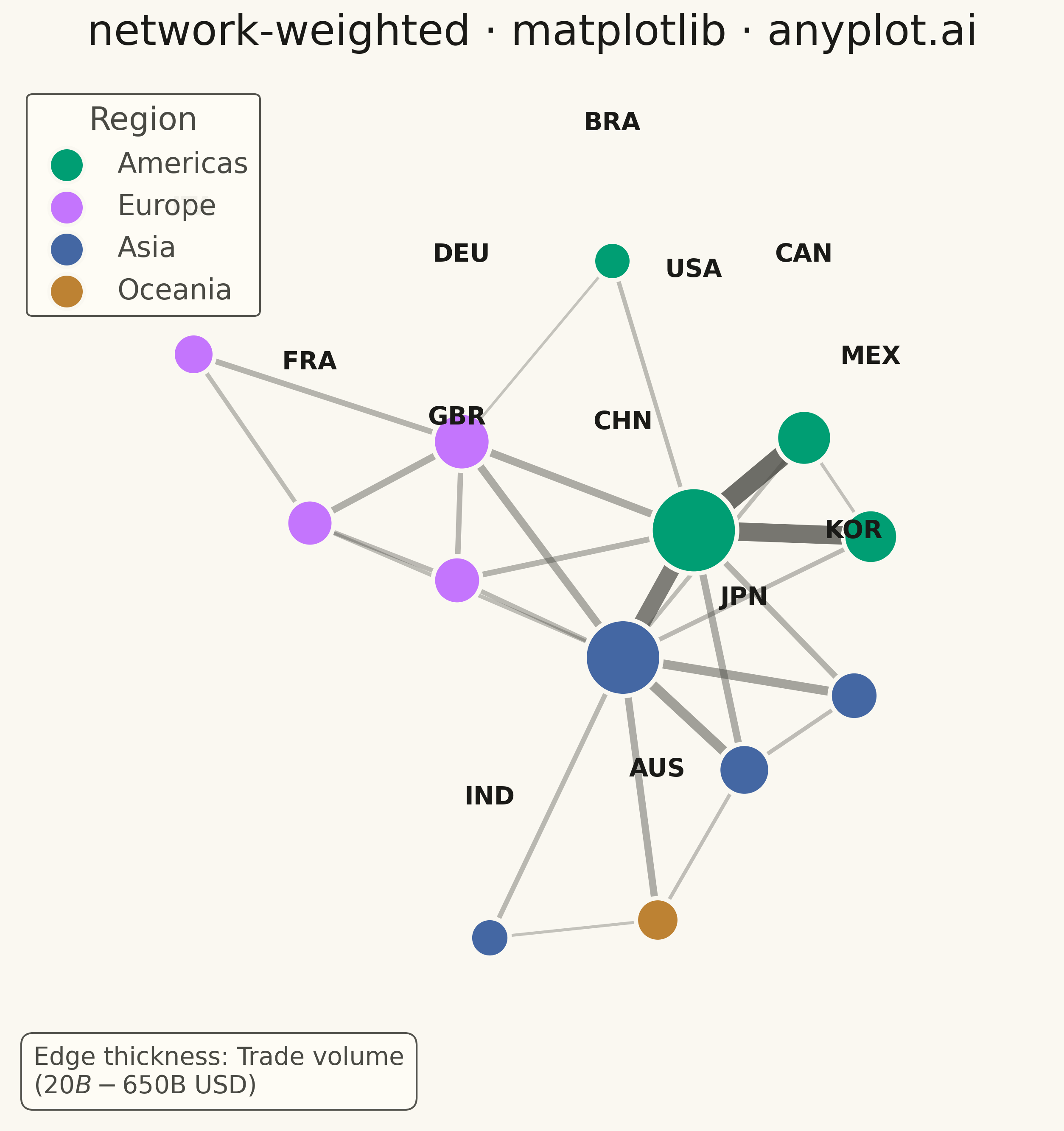
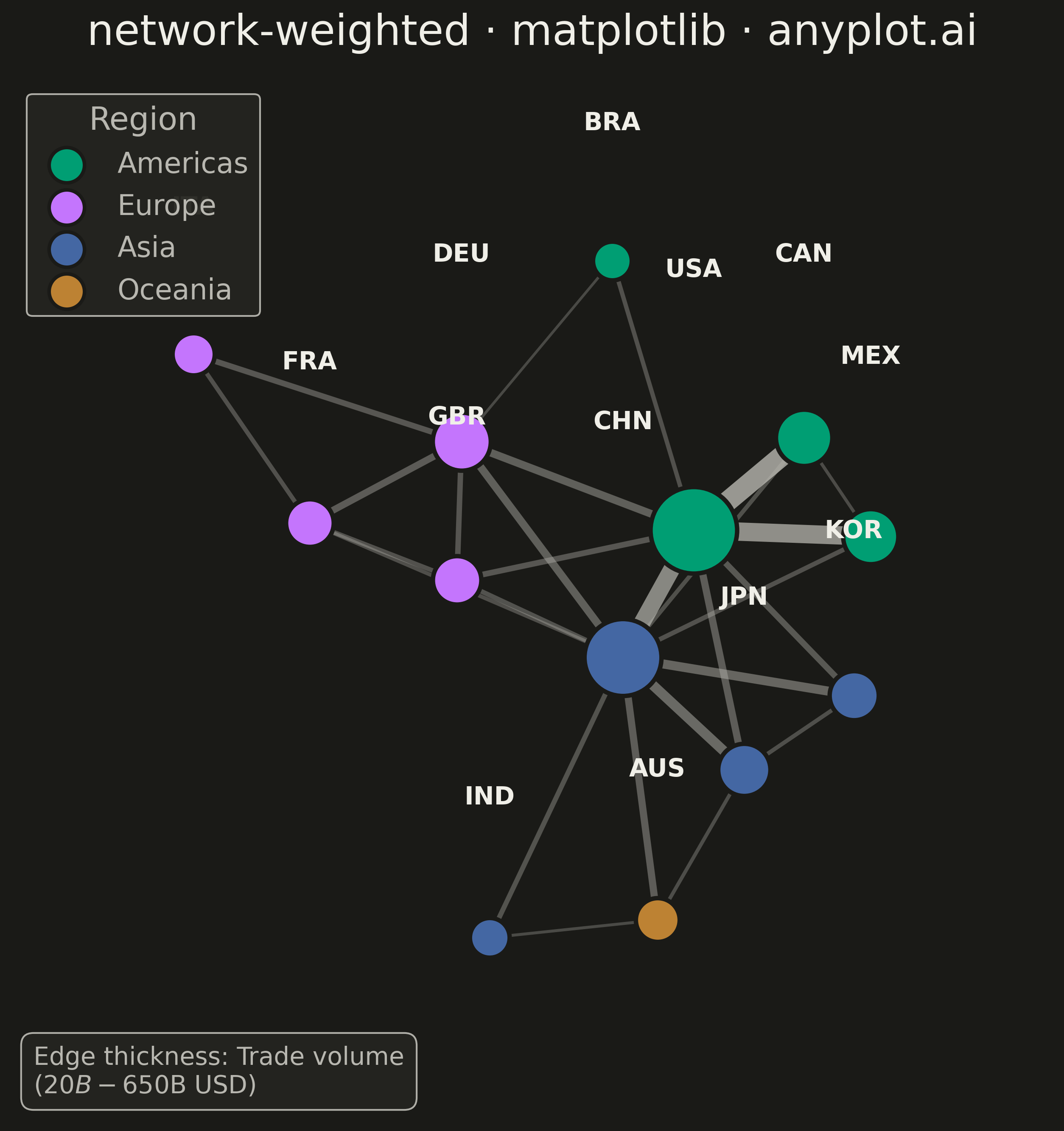
A weighted network graph displays relationships between entities using edge thickness to represent connection strength or weight. Unlike basic network graphs where edges are uniform, the varying line widths immediately communicate the relative importance of each relationship. This visualization makes it easy to identify strong vs weak connections, central hubs with many heavy links, and structural patterns in weighted relational data.
""" anyplot.ai
network-weighted: Weighted Network Graph with Edge Thickness
Library: matplotlib 3.10.9 | Python 3.13.13
Quality: 99/100 | Updated: 2026-05-17
"""

import os

import matplotlib.pyplot as plt
import numpy as np


# Theme tokens
THEME = os.getenv("ANYPLOT_THEME", "light")
PAGE_BG = "#FAF8F1" if THEME == "light" else "#1A1A17"
ELEVATED_BG = "#FFFDF6" if THEME == "light" else "#242420"
INK = "#1A1A17" if THEME == "light" else "#F0EFE8"
INK_SOFT = "#4A4A44" if THEME == "light" else "#B8B7B0"

# Okabe-Ito categorical palette (positions 1-4)
IMPRINT = ["#009E73", "#C475FD", "#4467A3", "#BD8233"]

# Data: Trade network between countries (billions USD)
np.random.seed(42)

# Define nodes (countries) with region groups
nodes = {
    "USA": {"group": 0},  # Americas
    "CAN": {"group": 0},
    "MEX": {"group": 0},
    "BRA": {"group": 0},
    "DEU": {"group": 1},  # Europe
    "FRA": {"group": 1},
    "GBR": {"group": 1},
    "ITA": {"group": 1},
    "CHN": {"group": 2},  # Asia
    "JPN": {"group": 2},
    "KOR": {"group": 2},
    "IND": {"group": 2},
    "AUS": {"group": 3},  # Oceania
}

# Define edges with trade volume weights (billions USD)
edges = [
    ("USA", "CAN", 650),
    ("USA", "MEX", 580),
    ("USA", "CHN", 520),
    ("USA", "JPN", 180),
    ("USA", "DEU", 200),
    ("USA", "GBR", 130),
    ("USA", "KOR", 140),
    ("USA", "BRA", 80),
    ("CAN", "CHN", 75),
    ("CAN", "MEX", 40),
    ("MEX", "CHN", 90),
    ("DEU", "FRA", 170),
    ("DEU", "GBR", 120),
    ("DEU", "ITA", 130),
    ("DEU", "CHN", 200),
    ("FRA", "GBR", 90),
    ("FRA", "ITA", 80),
    ("FRA", "CHN", 65),
    ("GBR", "CHN", 95),
    ("CHN", "JPN", 280),
    ("CHN", "KOR", 250),
    ("CHN", "AUS", 180),
    ("CHN", "IND", 100),
    ("JPN", "KOR", 70),
    ("JPN", "AUS", 55),
    ("IND", "AUS", 30),
    ("BRA", "DEU", 20),
]

# Force-directed layout computation
node_list = list(nodes.keys())
n = len(node_list)
node_idx = {name: i for i, name in enumerate(node_list)}

# Initialize positions randomly
pos = np.random.rand(n, 2) * 2 - 1

k = 1.5 / np.sqrt(n)  # Optimal distance
t = 0.5  # Temperature (step size)

for _ in range(300):
    disp = np.zeros((n, 2))

    # Repulsive forces between all pairs
    for i in range(n):
        for j in range(i + 1, n):
            delta = pos[i] - pos[j]
            dist = max(np.linalg.norm(delta), 0.01)
            force = k * k / dist * 1.5
            direction = delta / dist
            disp[i] += direction * force
            disp[j] -= direction * force

    # Attractive forces along edges (weighted)
    for src, tgt, weight in edges:
        i, j = node_idx[src], node_idx[tgt]
        delta = pos[i] - pos[j]
        dist = max(np.linalg.norm(delta), 0.01)
        force = dist * dist / k * (0.8 + weight / 400)
        direction = delta / dist
        disp[i] -= direction * force
        disp[j] += direction * force

    # Apply displacement with temperature limiting
    for i in range(n):
        disp_norm = max(np.linalg.norm(disp[i]), 0.01)
        pos[i] += disp[i] / disp_norm * min(disp_norm, t)

    t *= 0.97  # Cool down

# Normalize positions to [-1, 1]
pos_min = pos.min(axis=0)
pos_max = pos.max(axis=0)
pos = 2 * (pos - pos_min) / (pos_max - pos_min + 0.001) - 1
pos *= 0.75

positions = {name: pos[node_idx[name]] for name in node_list}

# Compute weighted degree for node sizing
weighted_degree = dict.fromkeys(nodes, 0)
for src, tgt, weight in edges:
    weighted_degree[src] += weight
    weighted_degree[tgt] += weight

# Region names and group mapping
region_names = ["Americas", "Europe", "Asia", "Oceania"]
group_colors = {i: IMPRINT[i] for i in range(4)}

# Create plot
fig, ax = plt.subplots(figsize=(16, 9), facecolor=PAGE_BG)
ax.set_facecolor(PAGE_BG)

# Edge width and alpha scaling
edge_weights = [w for _, _, w in edges]
max_weight = max(edge_weights)
min_weight = min(edge_weights)
weight_range = max_weight - min_weight

# Draw edges with varying thickness
for src, tgt, weight in edges:
    pos_src = positions[src]
    pos_tgt = positions[tgt]
    norm_w = (weight - min_weight) / weight_range if weight_range > 0 else 0.5
    line_width = 1.5 + norm_w * 10
    alpha = 0.3 + norm_w * 0.5
    ax.plot(
        [pos_src[0], pos_tgt[0]],
        [pos_src[1], pos_tgt[1]],
        color=INK_SOFT,
        linewidth=line_width,
        alpha=alpha,
        solid_capstyle="round",
        zorder=1,
    )

# Node sizes based on weighted degree
max_degree = max(weighted_degree.values())
node_sizes = {name: 400 + (weighted_degree[name] / max_degree) * 2000 for name in nodes}

# Draw nodes
for name, data in nodes.items():
    color = group_colors[data["group"]]
    node_pos = positions[name]
    ax.scatter(node_pos[0], node_pos[1], s=node_sizes[name], c=color, edgecolors=PAGE_BG, linewidths=2.5, zorder=2)

# Draw node labels (above nodes)
for name in nodes:
    node_pos = positions[name]
    node_radius = np.sqrt(node_sizes[name]) / 100
    ax.annotate(
        name,
        (node_pos[0], node_pos[1] + node_radius + 0.06),
        fontsize=14,
        fontweight="bold",
        ha="center",
        va="bottom",
        color=INK,
        zorder=3,
    )

# Region legend
legend_handles = []
for i, region in enumerate(region_names):
    handle = ax.scatter([], [], s=400, c=IMPRINT[i], edgecolors=PAGE_BG, linewidths=2, label=region)
    legend_handles.append(handle)

leg = ax.legend(
    handles=legend_handles, loc="upper left", fontsize=16, framealpha=0.95, title="Region", title_fontsize=18
)
if leg:
    leg.get_frame().set_facecolor(ELEVATED_BG)
    leg.get_frame().set_edgecolor(INK_SOFT)
    plt.setp(leg.get_texts(), color=INK_SOFT)
    plt.setp(leg.get_title(), color=INK_SOFT)

# Edge thickness legend
legend_text = f"Edge thickness: Trade volume\n(${min_weight}B - ${max_weight}B USD)"
ax.annotate(
    legend_text,
    xy=(0.02, 0.02),
    xycoords="axes fraction",
    fontsize=14,
    bbox={"boxstyle": "round,pad=0.5", "facecolor": ELEVATED_BG, "edgecolor": INK_SOFT, "alpha": 0.95},
    verticalalignment="bottom",
    color=INK_SOFT,
)

# Style
ax.set_title("network-weighted · matplotlib · anyplot.ai", fontsize=24, fontweight="medium", color=INK, pad=20)
ax.set_xlim(-1.15, 1.15)
ax.set_ylim(-1.15, 1.15)
ax.set_aspect("equal")
ax.axis("off")

plt.tight_layout()
plt.savefig(f"plot-{THEME}.png", dpi=300, bbox_inches="tight", facecolor=PAGE_BG)
Runnable source as JSON, for any HTTP client: https://api.anyplot.ai/specs/network-weighted/matplotlib/code. Any spec id and library id listed in llms-full.txt fit the same URL shape; every URL below is complete and callable.
{
  "spec_id": "network-weighted",
  "language": "python",
  "library": "matplotlib",
  "page": "https://anyplot.ai/network-weighted/python/matplotlib",
  "hub": "https://anyplot.ai/network-weighted",
  "code_json": "https://api.anyplot.ai/specs/network-weighted/matplotlib/code",
  "spec_json": "https://api.anyplot.ai/specs/network-weighted",
  "render_light_png": "https://storage.googleapis.com/anyplot-images/plots/network-weighted/python/matplotlib/plot-light.png",
  "render_dark_png": "https://storage.googleapis.com/anyplot-images/plots/network-weighted/python/matplotlib/plot-dark.png",
  "quality_score": 99.0,
  "license": "MIT",
  "guide": "https://anyplot.ai/llms.txt"
}
Part of Weighted Network Graph with Edge Thickness on anyplot.ai.