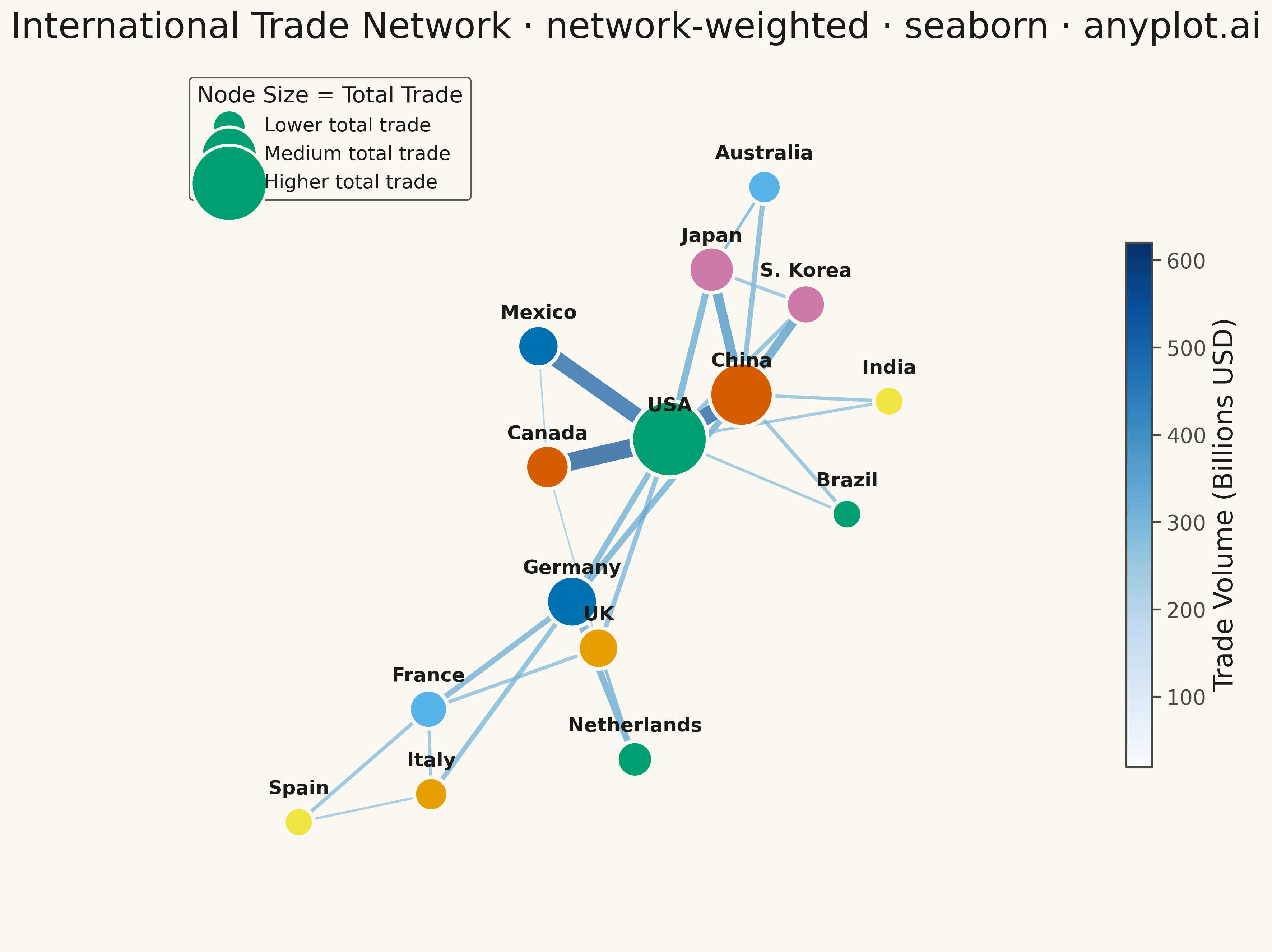
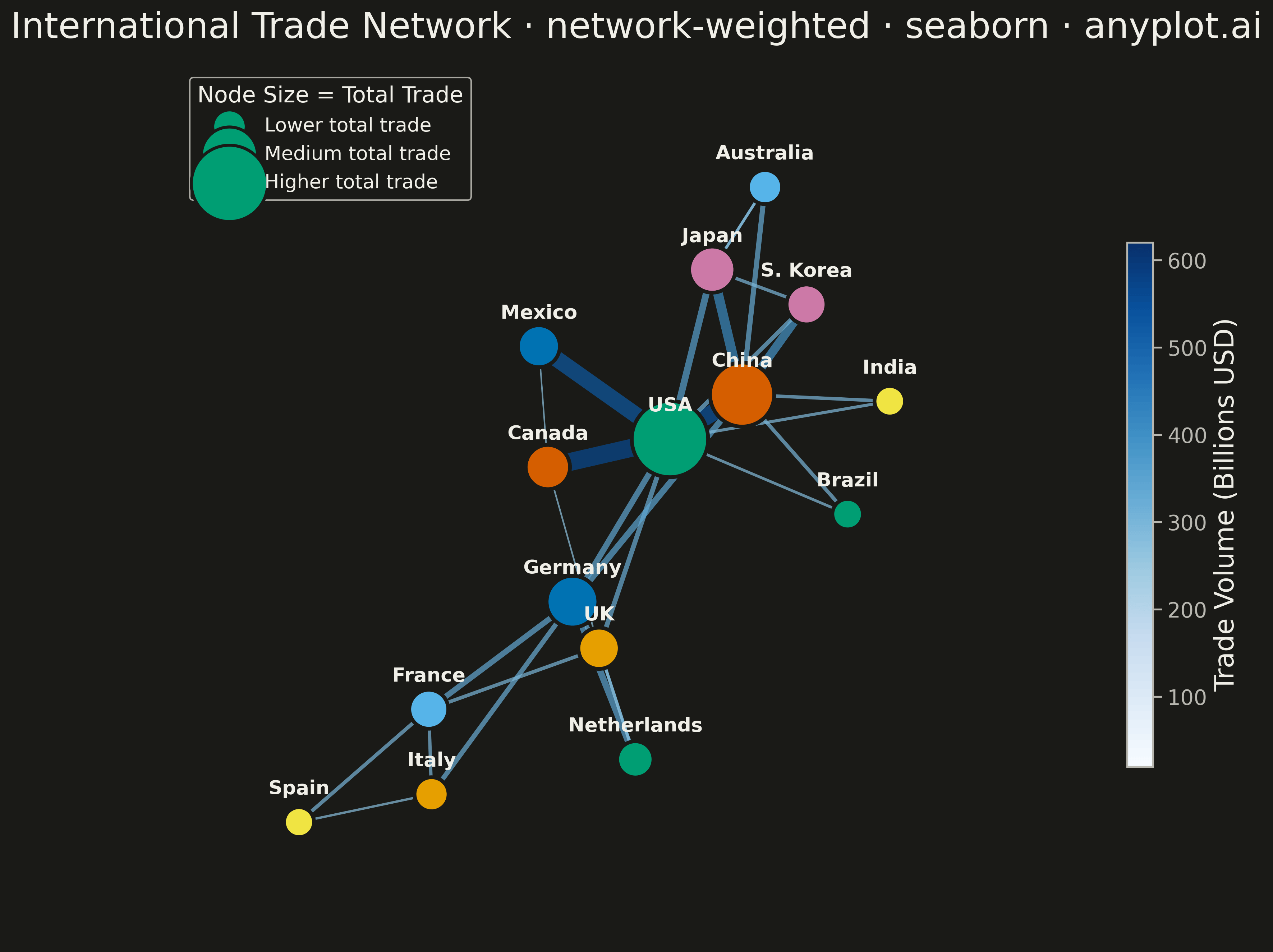
A weighted network graph displays relationships between entities using edge thickness to represent connection strength or weight. Unlike basic network graphs where edges are uniform, the varying line widths immediately communicate the relative importance of each relationship. This visualization makes it easy to identify strong vs weak connections, central hubs with many heavy links, and structural patterns in weighted relational data.
""" anyplot.ai
network-weighted: Weighted Network Graph with Edge Thickness
Library: seaborn 0.13.2 | Python 3.13.13
Quality: 70/100 | Updated: 2026-05-17
"""

import matplotlib.pyplot as plt
import numpy as np
import seaborn as sns
from matplotlib.collections import LineCollection


# Set seaborn style for consistent aesthetics
sns.set_style("whitegrid")
sns.set_context("talk", font_scale=1.2)

# Data: Trade network between countries (billions USD annual trade volume)
np.random.seed(42)

# Define nodes (15 countries as trading partners)
countries = [
    "USA",
    "China",
    "Germany",
    "Japan",
    "UK",
    "France",
    "India",
    "Brazil",
    "Canada",
    "Mexico",
    "S. Korea",
    "Italy",
    "Australia",
    "Spain",
    "Netherlands",
]
n_nodes = len(countries)
node_idx = {name: i for i, name in enumerate(countries)}

# Create weighted edges (source, target, weight in billions USD)
edges_data = [
    ("USA", "China", 580),
    ("USA", "Canada", 620),
    ("USA", "Mexico", 550),
    ("USA", "Japan", 210),
    ("USA", "Germany", 180),
    ("USA", "UK", 140),
    ("China", "Japan", 320),
    ("China", "S. Korea", 280),
    ("China", "Germany", 190),
    ("China", "Australia", 150),
    ("China", "India", 90),
    ("Germany", "France", 170),
    ("Germany", "Netherlands", 200),
    ("Germany", "UK", 130),
    ("Germany", "Italy", 140),
    ("Japan", "S. Korea", 85),
    ("Japan", "Australia", 70),
    ("UK", "France", 95),
    ("UK", "Netherlands", 80),
    ("France", "Italy", 85),
    ("France", "Spain", 100),
    ("India", "USA", 75),
    ("Brazil", "USA", 65),
    ("Brazil", "China", 100),
    ("Canada", "UK", 25),
    ("Mexico", "Canada", 20),
    ("Australia", "Japan", 60),
    ("S. Korea", "USA", 120),
    ("Netherlands", "UK", 70),
    ("Italy", "Spain", 50),
]

# Build edge list with indices
edges = [(node_idx[s], node_idx[t], w) for s, t, w in edges_data]

# Calculate weighted degree for node sizing
weighted_degrees = np.zeros(n_nodes)
for i, j, w in edges:
    weighted_degrees[i] += w
    weighted_degrees[j] += w

# Spring layout using Fruchterman-Reingold algorithm (inline implementation)
np.random.seed(42)
pos = np.random.rand(n_nodes, 2) * 2 - 1
area = 4.0
k_rep = np.sqrt(area / n_nodes) * 0.8

for iteration in range(300):
    # Calculate repulsive forces between all pairs
    disp = np.zeros((n_nodes, 2))
    for i in range(n_nodes):
        for j in range(i + 1, n_nodes):
            delta = pos[i] - pos[j]
            dist = max(np.linalg.norm(delta), 0.01)
            force = k_rep**2 / dist
            direction = delta / dist
            disp[i] += direction * force
            disp[j] -= direction * force

    # Calculate attractive forces along edges
    for i, j, w in edges:
        delta = pos[i] - pos[j]
        dist = max(np.linalg.norm(delta), 0.01)
        force = dist**2 / k_rep * (1 + w / 300)
        direction = delta / dist
        disp[i] -= direction * force
        disp[j] += direction * force

    # Limit displacement and update positions
    temp = 0.1 * (1 - iteration / 300)
    for i in range(n_nodes):
        disp_norm = max(np.linalg.norm(disp[i]), 0.01)
        pos[i] += disp[i] / disp_norm * min(disp_norm, temp)
        pos[i] = np.clip(pos[i], -1, 1)

# Scale positions to canvas
positions = pos * 0.8

# Prepare edge data
edge_weights = [w for _, _, w in edges]
min_weight, max_weight = min(edge_weights), max(edge_weights)
edge_widths = [1 + (w - min_weight) / (max_weight - min_weight) * 11 for w in edge_weights]
edge_colors_norm = [(w - min_weight) / (max_weight - min_weight) for w in edge_weights]

# Scale node sizes based on weighted degree
node_sizes = (
    400 + (weighted_degrees - weighted_degrees.min()) / (weighted_degrees.max() - weighted_degrees.min()) * 2200
)

# Create figure
fig, ax = plt.subplots(figsize=(16, 9))

# Create color palette for edges using seaborn
edge_cmap = sns.color_palette("Blues", as_cmap=True)

# Draw edges as LineCollection for proper width variation
segments = []
colors = []
widths = []
for idx, (i, j, _w) in enumerate(edges):
    segments.append([positions[i], positions[j]])
    colors.append(edge_cmap(edge_colors_norm[idx]))
    widths.append(edge_widths[idx])

lc = LineCollection(segments, colors=colors, linewidths=widths, alpha=0.7, zorder=1)
ax.add_collection(lc)

# Node colors using seaborn palette
node_palette = sns.color_palette("Set2", n_colors=n_nodes)

# Draw nodes
ax.scatter(positions[:, 0], positions[:, 1], s=node_sizes, c=node_palette, edgecolors="white", linewidths=2.5, zorder=2)

# Draw labels with offset to avoid overlap with nodes
for i, name in enumerate(countries):
    ax.annotate(
        name,
        (positions[i, 0], positions[i, 1] + 0.06),
        fontsize=13,
        fontweight="bold",
        color="#333333",
        ha="center",
        va="bottom",
        zorder=3,
    )

# Add colorbar for edge weights
sm = plt.cm.ScalarMappable(cmap=edge_cmap, norm=plt.Normalize(vmin=min_weight, vmax=max_weight))
sm.set_array([])
cbar = plt.colorbar(sm, ax=ax, shrink=0.6, pad=0.02)
cbar.set_label("Trade Volume (Billions USD)", fontsize=18)
cbar.ax.tick_params(labelsize=14)

# Add legend for node size interpretation
legend_elements = [
    plt.scatter([], [], s=500, c="#66c2a5", edgecolors="white", linewidths=2, label="Lower total trade"),
    plt.scatter([], [], s=1400, c="#66c2a5", edgecolors="white", linewidths=2, label="Medium total trade"),
    plt.scatter([], [], s=2600, c="#66c2a5", edgecolors="white", linewidths=2, label="Higher total trade"),
]
ax.legend(
    handles=legend_elements,
    loc="upper left",
    fontsize=13,
    title="Node Size = Total Trade",
    title_fontsize=15,
    framealpha=0.9,
)

# Style
ax.set_title("International Trade Network · network-weighted · seaborn · pyplots.ai", fontsize=24, pad=20)
ax.set_xlim(-1.1, 1.2)
ax.set_ylim(-1.1, 1.1)
ax.axis("off")
ax.set_aspect("equal")

plt.tight_layout()
plt.savefig("plot.png", dpi=300, bbox_inches="tight", facecolor="white")
Runnable source as JSON, for any HTTP client: https://api.anyplot.ai/specs/network-weighted/seaborn/code. Any spec id and library id listed in llms-full.txt fit the same URL shape; every URL below is complete and callable.
{
  "spec_id": "network-weighted",
  "language": "python",
  "library": "seaborn",
  "page": "https://anyplot.ai/network-weighted/python/seaborn",
  "hub": "https://anyplot.ai/network-weighted",
  "code_json": "https://api.anyplot.ai/specs/network-weighted/seaborn/code",
  "spec_json": "https://api.anyplot.ai/specs/network-weighted",
  "render_light_png": "https://storage.googleapis.com/anyplot-images/plots/network-weighted/python/seaborn/plot-light.png",
  "render_dark_png": "https://storage.googleapis.com/anyplot-images/plots/network-weighted/python/seaborn/plot-dark.png",
  "quality_score": 70.0,
  "license": "MIT",
  "guide": "https://anyplot.ai/llms.txt"
}
Part of Weighted Network Graph with Edge Thickness on anyplot.ai.