The same plot in 14 other libraries — JavaScript: Chart.js, Apache ECharts, Highcharts, MUI X Charts; Python: Altair, Bokeh, lets-plot, Matplotlib, Plotly, plotnine, Pygal, Seaborn; R: ggplot2; Julia: Makie.jl. Compare all 15 side by side: Basic Q-Q Plot in Python, R, Julia and JavaScript.
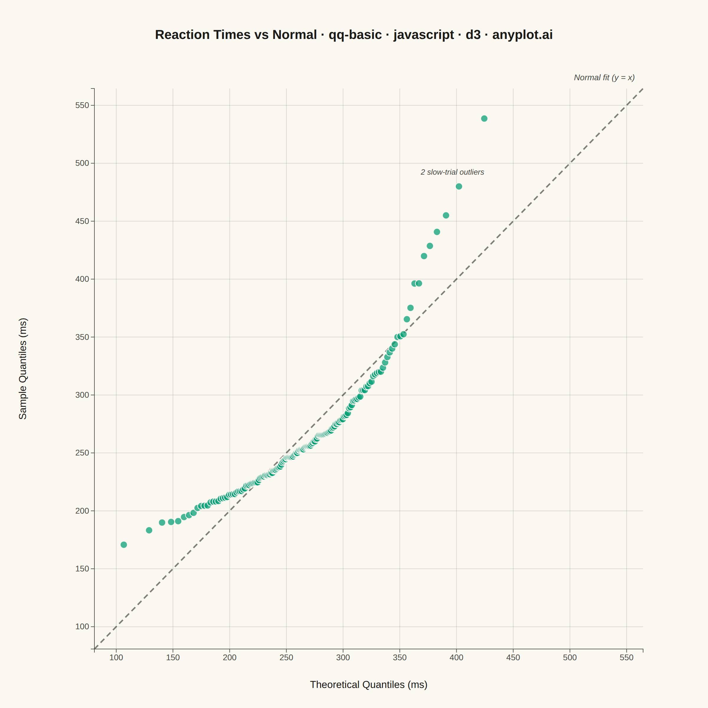
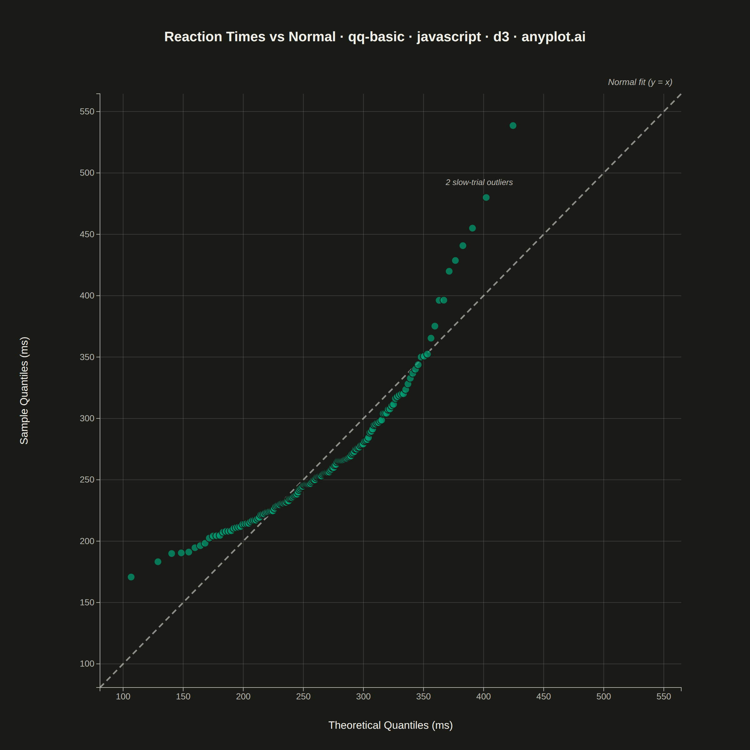
A Q-Q (Quantile-Quantile) plot compares the distribution of a dataset against a theoretical distribution (typically normal) or another dataset. Points are plotted by matching sample quantiles to theoretical quantiles, with a reference line indicating perfect distribution match. Deviations from the line reveal distribution characteristics such as skewness, heavy tails, and outliers.
// anyplot.ai
// qq-basic: Basic Q-Q Plot
// Library: d3 7.9.0 | JavaScript 22.23.1
// Quality: 89/100 | Created: 2026-07-24
//# anyplot-orientation: square

// --- Theme + mount ------------------------------------------------------
const t = window.ANYPLOT_TOKENS;
const { width, height } = window.ANYPLOT_SIZE;

// --- Deterministic RNG (mulberry32) + standard-normal sampling ----------
function mulberry32(seed) {
  let s = seed >>> 0;
  return function () {
    s = (s + 0x6d2b79f5) | 0;
    let x = Math.imul(s ^ (s >>> 15), 1 | s);
    x = (x + Math.imul(x ^ (x >>> 7), 61 | x)) ^ x;
    return ((x ^ (x >>> 14)) >>> 0) / 4294967296;
  };
}

// Acklam's rational approximation of the standard-normal inverse CDF (probit).
function probit(p) {
  const a = [-3.969683028665376e1, 2.209460984245205e2, -2.759285104469687e2, 1.38357751867269e2, -3.066479806614716e1, 2.506628277459239];
  const b = [-5.447609879822406e1, 1.615858368580409e2, -1.556989798598866e2, 6.680131188771972e1, -1.328068155288572e1];
  const c = [-7.784894002430293e-3, -3.223964580411365e-1, -2.400758277161838, -2.549732539343734, 4.374664141464968, 2.938163982698783];
  const d = [7.784695709041462e-3, 3.224671290700398e-1, 2.445134137142996, 3.754408661907416];
  const pLow = 0.02425;
  if (p < pLow) {
    const q = Math.sqrt(-2 * Math.log(p));
    return (((((c[0] * q + c[1]) * q + c[2]) * q + c[3]) * q + c[4]) * q + c[5]) / ((((d[0] * q + d[1]) * q + d[2]) * q + d[3]) * q + 1);
  }
  if (p <= 1 - pLow) {
    const q = p - 0.5;
    const r = q * q;
    return ((((( a[0] * r + a[1]) * r + a[2]) * r + a[3]) * r + a[4]) * r + a[5]) * q / (((((b[0] * r + b[1]) * r + b[2]) * r + b[3]) * r + b[4]) * r + 1);
  }
  const q = Math.sqrt(-2 * Math.log(1 - p));
  return -(((((c[0] * q + c[1]) * q + c[2]) * q + c[3]) * q + c[4]) * q + c[5]) / ((((d[0] * q + d[1]) * q + d[2]) * q + d[3]) * q + 1);
}

// --- Data: reaction times (ms) from a cognitive-experiment trial --------
// Right-skewed by construction (typical of RT data) so the sample visibly
// bows away from the normal reference line in the upper tail, plus two
// explicit slow-trial outliers.
const rng = mulberry32(20260724);
const MU0 = 250;
const SIGMA0 = 35;
const SKEW = 20;
const n0 = 158;
const sample = [];
for (let i = 0; i < n0; i += 2) {
  const u1 = rng();
  const u2 = rng();
  const mag = Math.sqrt(-2 * Math.log(u1));
  const z0 = mag * Math.cos(2 * Math.PI * u2);
  const z1 = mag * Math.sin(2 * Math.PI * u2);
  for (const z of [z0, z1]) {
    const value = MU0 + SIGMA0 * z + SKEW * Math.max(z, 0) ** 2;
    sample.push(value);
  }
}
sample.push(455, 480); // two slow-trial outliers
sample.sort((a, b) => a - b);

const n = sample.length;
const muHat = d3.mean(sample);
const sigmaHat = d3.deviation(sample);
const points = sample.map((value, i) => {
  const p = (i + 0.5) / n;
  return { theoretical: muHat + sigmaHat * probit(p), sample: value };
});

// --- Layout ---------------------------------------------------------------
// Equal left+right / top+bottom margin sums keep the plot area square so the
// y = x reference line renders at a true visual 45°.
const margin = { top: 150, right: 110, bottom: 100, left: 160 };
const iw = width - margin.left - margin.right;
const ih = height - margin.top - margin.bottom;

// --- Scales -----------------------------------------------------------------
const allValues = points.flatMap((d) => [d.theoretical, d.sample]);
const [rawMin, rawMax] = d3.extent(allValues);
const pad = (rawMax - rawMin) * 0.06;
const domain = [rawMin - pad, rawMax + pad];

const x = d3.scaleLinear().domain(domain).range([0, iw]);
const y = d3.scaleLinear().domain(domain).range([ih, 0]);

// --- SVG mount --------------------------------------------------------------
const svg = d3.select("#container").append("svg").attr("width", width).attr("height", height);
const g = svg.append("g").attr("transform", `translate(${margin.left},${margin.top})`);

// --- Gridlines (both axes, subtle) ------------------------------------------
g.append("g")
  .attr("transform", `translate(0,${ih})`)
  .call(d3.axisBottom(x).ticks(7).tickSize(-ih).tickFormat(""))
  .call((sel) => sel.select(".domain").remove())
  .selectAll("line")
  .attr("stroke", t.grid);

g.append("g")
  .call(d3.axisLeft(y).ticks(7).tickSize(-iw).tickFormat(""))
  .call((sel) => sel.select(".domain").remove())
  .selectAll("line")
  .attr("stroke", t.grid);

// --- Reference line y = x (normal distribution fit to the sample) ----------
g.append("line")
  .attr("x1", x(domain[0]))
  .attr("y1", y(domain[0]))
  .attr("x2", x(domain[1]))
  .attr("y2", y(domain[1]))
  .attr("stroke", t.ink)
  .attr("stroke-width", 2.5)
  .attr("stroke-dasharray", "9,6")
  .attr("opacity", 0.55);

g.append("text")
  .attr("x", x(domain[1]) - 14)
  .attr("y", y(domain[1]) - 14)
  .attr("text-anchor", "end")
  .attr("fill", t.inkSoft)
  .style("font-size", "14px")
  .style("font-style", "italic")
  .text("Normal fit (y = x)");

// --- Sample points ------------------------------------------------------
g.selectAll("circle")
  .data(points)
  .join("circle")
  .attr("cx", (d) => x(d.theoretical))
  .attr("cy", (d) => y(d.sample))
  .attr("r", 6)
  .attr("fill", t.palette[0])
  .attr("fill-opacity", 0.72)
  .attr("stroke", t.pageBg)
  .attr("stroke-width", 1.2);

// --- Outlier callout (the two explicit slow-trial outliers) ----------------
const outlierValues = [455, 480];
const outlierPts = points.filter((d) => outlierValues.includes(d.sample));
const outlierCx = d3.mean(outlierPts, (d) => x(d.theoretical));
const outlierTopY = d3.min(outlierPts, (d) => y(d.sample));
g.append("text")
  .attr("x", outlierCx)
  .attr("y", outlierTopY - 20)
  .attr("text-anchor", "middle")
  .attr("fill", t.inkSoft)
  .style("font-size", "13px")
  .style("font-style", "italic")
  .text("2 slow-trial outliers");

// --- Axes ----------------------------------------------------------------
const xAxis = g.append("g").attr("transform", `translate(0,${ih})`).call(d3.axisBottom(x).ticks(7));
const yAxis = g.append("g").call(d3.axisLeft(y).ticks(7));
for (const ax of [xAxis, yAxis]) {
  ax.selectAll("text").attr("fill", t.inkSoft).style("font-size", "14px");
  ax.selectAll("line").attr("stroke", t.inkSoft);
  ax.select(".domain").attr("stroke", t.inkSoft);
}

// --- Axis labels -----------------------------------------------------------
svg.append("text")
  .attr("x", margin.left + iw / 2)
  .attr("y", height - 34)
  .attr("text-anchor", "middle")
  .attr("fill", t.ink)
  .style("font-size", "17px")
  .text("Theoretical Quantiles (ms)");

svg.append("text")
  .attr("transform", `translate(${44},${margin.top + ih / 2}) rotate(-90)`)
  .attr("text-anchor", "middle")
  .attr("fill", t.ink)
  .style("font-size", "17px")
  .text("Sample Quantiles (ms)");

// --- Title -------------------------------------------------------------
const title = "Reaction Times vs Normal · qq-basic · javascript · d3 · anyplot.ai";
const titleFontSize = Math.round(22 * Math.min(1, 67 / title.length));
svg.append("text")
  .attr("x", width / 2)
  .attr("y", 66)
  .attr("text-anchor", "middle")
  .attr("fill", t.ink)
  .style("font-size", `${titleFontSize}px`)
  .style("font-weight", "600")
  .text(title);
Runnable source as JSON, for any HTTP client: https://api.anyplot.ai/specs/qq-basic/d3/code. Any spec id and library id listed in llms-full.txt fit the same URL shape; every URL below is complete and callable.
{
  "spec_id": "qq-basic",
  "language": "javascript",
  "library": "d3",
  "page": "https://anyplot.ai/qq-basic/javascript/d3",
  "hub": "https://anyplot.ai/qq-basic",
  "code_json": "https://api.anyplot.ai/specs/qq-basic/d3/code",
  "spec_json": "https://api.anyplot.ai/specs/qq-basic",
  "render_light_png": "https://storage.googleapis.com/anyplot-images/plots/qq-basic/javascript/d3/plot-light.png",
  "render_dark_png": "https://storage.googleapis.com/anyplot-images/plots/qq-basic/javascript/d3/plot-dark.png",
  "interactive_light_html": "https://storage.googleapis.com/anyplot-images/plots/qq-basic/javascript/d3/plot-light.html",
  "interactive_dark_html": "https://storage.googleapis.com/anyplot-images/plots/qq-basic/javascript/d3/plot-dark.html",
  "quality_score": 89.0,
  "license": "MIT",
  "guide": "https://anyplot.ai/llms.txt"
}
Part of Basic Q-Q Plot on anyplot.ai.