The same plot in 14 other libraries — Python: Altair, Bokeh, lets-plot, Matplotlib, Plotly, plotnine, Pygal, Seaborn; R: ggplot2; JavaScript: Chart.js, D3.js, Apache ECharts, Highcharts, MUI X Charts. Compare all 15 side by side: Basic Q-Q Plot in Python, R, Julia and JavaScript.
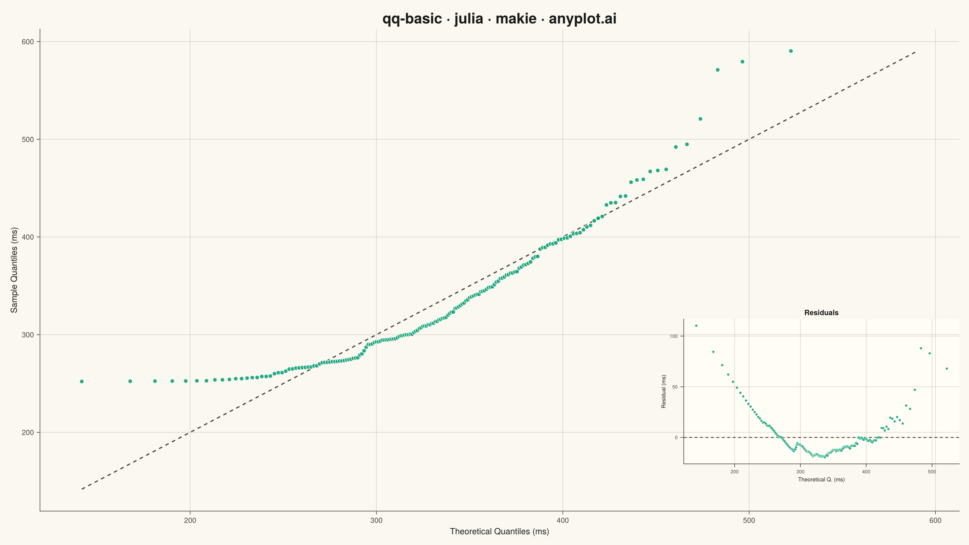
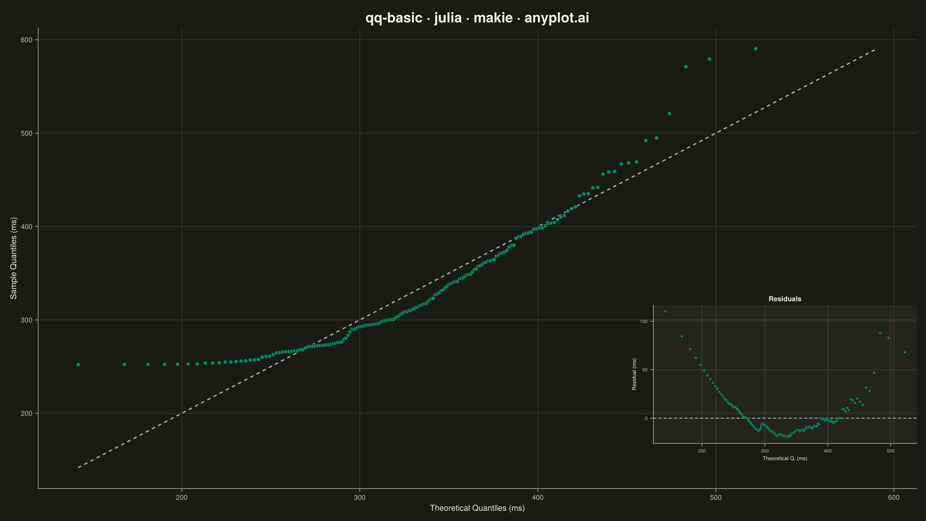
A Q-Q (Quantile-Quantile) plot compares the distribution of a dataset against a theoretical distribution (typically normal) or another dataset. Points are plotted by matching sample quantiles to theoretical quantiles, with a reference line indicating perfect distribution match. Deviations from the line reveal distribution characteristics such as skewness, heavy tails, and outliers.
# anyplot.ai
# qq-basic: Basic Q-Q Plot
# Library: makie 0.21.9 | Julia 1.11.9
# Quality: 89/100 | Created: 2026-07-24

using CairoMakie
using Colors
using Random
using Statistics

Random.seed!(42)

# --- Theme tokens ------------------------------------------------------------
const THEME       = get(ENV, "ANYPLOT_THEME", "light")
const PAGE_BG     = THEME == "light" ? colorant"#FAF8F1" : colorant"#1A1A17"
const ELEVATED_BG = THEME == "light" ? colorant"#FFFDF6" : colorant"#242420"
const INK         = THEME == "light" ? colorant"#1A1A17" : colorant"#F0EFE8"
const INK_SOFT    = THEME == "light" ? colorant"#4A4A44" : colorant"#B8B7B0"
const IMPRINT_PALETTE = [
    colorant"#009E73", colorant"#C475FD", colorant"#4467A3", colorant"#BD8233",
    colorant"#AE3030", colorant"#2ABCCD", colorant"#954477", colorant"#99B314",
]

# --- Standard normal quantile (inverse CDF), Acklam's rational approximation --
function norm_quantile(p)
    a = (-3.969683028665376e+01, 2.209460984245205e+02, -2.759285104469687e+02,
        1.383577518672690e+02, -3.066479806614716e+01, 2.506628277459239e+00)
    b = (-5.447609879822406e+01, 1.615858368580409e+02, -1.556989798598866e+02,
        6.680131188771972e+01, -1.328068155288572e+01)
    c = (-7.784894002430293e-03, -3.223964580411365e-01, -2.400758277161838e+00,
        -2.549732539343734e+00, 4.374664141464968e+00, 2.938163982698783e+00)
    d = (7.784695709041462e-03, 3.224671290700398e-01, 2.445134137142996e+00,
        3.754408661907416e+00)
    p_low = 0.02425
    p_high = 1 - p_low
    if p < p_low
        q = sqrt(-2 * log(p))
        return (((((c[1] * q + c[2]) * q + c[3]) * q + c[4]) * q + c[5]) * q + c[6]) /
               ((((d[1] * q + d[2]) * q + d[3]) * q + d[4]) * q + 1)
    elseif p <= p_high
        q = p - 0.5
        r = q * q
        return (((((a[1] * r + a[2]) * r + a[3]) * r + a[4]) * r + a[5]) * r + a[6]) * q /
               (((((b[1] * r + b[2]) * r + b[3]) * r + b[4]) * r + b[5]) * r + 1)
    else
        q = sqrt(-2 * log(1 - p))
        return -(((((c[1] * q + c[2]) * q + c[3]) * q + c[4]) * q + c[5]) * q + c[6]) /
               ((((d[1] * q + d[2]) * q + d[3]) * q + d[4]) * q + 1)
    end
end

# --- Data ----------------------------------------------------------------
# Reaction times (ms) from a simple cognitive task. Response-time data is
# classically right-skewed, giving the Q-Q plot a clear upward curve away
# from the reference line at the high end — a textbook normality check.
n = 180
z = randn(n)
reaction_times_ms = 320.0 .+ 70.0 .* z .+ 18.0 .* z .^ 2

sample_q = sort(reaction_times_ms)
mu, sigma = mean(sample_q), std(sample_q)
plot_pos = ((1:n) .- 0.5) ./ n
theoretical_q = mu .+ sigma .* norm_quantile.(plot_pos)

lo = min(minimum(theoretical_q), minimum(sample_q))
hi = max(maximum(theoretical_q), maximum(sample_q))
residual_ms = sample_q .- theoretical_q

# --- Plot ------------------------------------------------------------------
title_str = "qq-basic · julia · makie · anyplot.ai"

fig = Figure(size = (1600, 900), fontsize = 14, backgroundcolor = PAGE_BG)

ax = Axis(
    fig[1, 1];
    title             = title_str,
    titlesize         = 24,
    titlecolor        = INK,
    xlabel            = "Theoretical Quantiles (ms)",
    ylabel            = "Sample Quantiles (ms)",
    xlabelsize        = 14,
    ylabelsize        = 14,
    xticklabelsize    = 12,
    yticklabelsize    = 12,
    xlabelcolor       = INK,
    ylabelcolor       = INK,
    xticklabelcolor   = INK_SOFT,
    yticklabelcolor   = INK_SOFT,
    xtickcolor        = INK_SOFT,
    ytickcolor        = INK_SOFT,
    backgroundcolor   = PAGE_BG,
    topspinevisible   = false,
    rightspinevisible = false,
    leftspinecolor    = INK_SOFT,
    bottomspinecolor  = INK_SOFT,
    xgridcolor        = RGBAf(INK.r, INK.g, INK.b, 0.15),
    ygridcolor        = RGBAf(INK.r, INK.g, INK.b, 0.15),
    xminorgridvisible = false,
    yminorgridvisible = false,
)

lines!(ax, [lo, hi], [lo, hi]; color = INK_SOFT, linewidth = 2.0, linestyle = :dash)
scatter!(ax, theoretical_q, sample_q;
    color = (IMPRINT_PALETTE[1], 0.85), markersize = 10, strokewidth = 1.0, strokecolor = PAGE_BG)

# --- Residual inset: a Makie-native nested Axis sharing the same grid cell,
# positioned in the corner farthest from the diagonal band, to show the
# skew signature (sample - theoretical) as a companion diagnostic panel.
ax_inset = Axis(
    fig[1, 1];
    width             = Relative(0.30),
    height            = Relative(0.30),
    halign            = 1.0,
    valign            = 0.14,
    title             = "Residuals",
    titlesize         = 12,
    titlecolor        = INK,
    xlabel            = "Theoretical Q. (ms)",
    ylabel            = "Residual (ms)",
    xlabelsize        = 9,
    ylabelsize        = 9,
    xticklabelsize    = 8,
    yticklabelsize    = 8,
    xlabelcolor       = INK,
    ylabelcolor       = INK,
    xticklabelcolor   = INK_SOFT,
    yticklabelcolor   = INK_SOFT,
    xtickcolor        = INK_SOFT,
    ytickcolor        = INK_SOFT,
    backgroundcolor   = ELEVATED_BG,
    topspinevisible   = false,
    rightspinevisible = false,
    leftspinecolor    = INK_SOFT,
    bottomspinecolor  = INK_SOFT,
    xgridcolor        = RGBAf(INK.r, INK.g, INK.b, 0.15),
    ygridcolor        = RGBAf(INK.r, INK.g, INK.b, 0.15),
    xminorgridvisible = false,
    yminorgridvisible = false,
)

hlines!(ax_inset, [0.0]; color = INK_SOFT, linewidth = 1.5, linestyle = :dash)
scatter!(ax_inset, theoretical_q, residual_ms;
    color = (IMPRINT_PALETTE[1], 0.85), markersize = 6, strokewidth = 0.5, strokecolor = ELEVATED_BG)

# --- Save --------------------------------------------------------------------
save("plot-$(THEME).png", fig; px_per_unit = 2)
Runnable source as JSON, for any HTTP client: https://api.anyplot.ai/specs/qq-basic/makie/code. Any spec id and library id listed in llms-full.txt fit the same URL shape; every URL below is complete and callable.
{
  "spec_id": "qq-basic",
  "language": "julia",
  "library": "makie",
  "page": "https://anyplot.ai/qq-basic/julia/makie",
  "hub": "https://anyplot.ai/qq-basic",
  "code_json": "https://api.anyplot.ai/specs/qq-basic/makie/code",
  "spec_json": "https://api.anyplot.ai/specs/qq-basic",
  "render_light_png": "https://storage.googleapis.com/anyplot-images/plots/qq-basic/julia/makie/plot-light.png",
  "render_dark_png": "https://storage.googleapis.com/anyplot-images/plots/qq-basic/julia/makie/plot-dark.png",
  "quality_score": 89.0,
  "license": "MIT",
  "guide": "https://anyplot.ai/llms.txt"
}
Part of Basic Q-Q Plot on anyplot.ai.