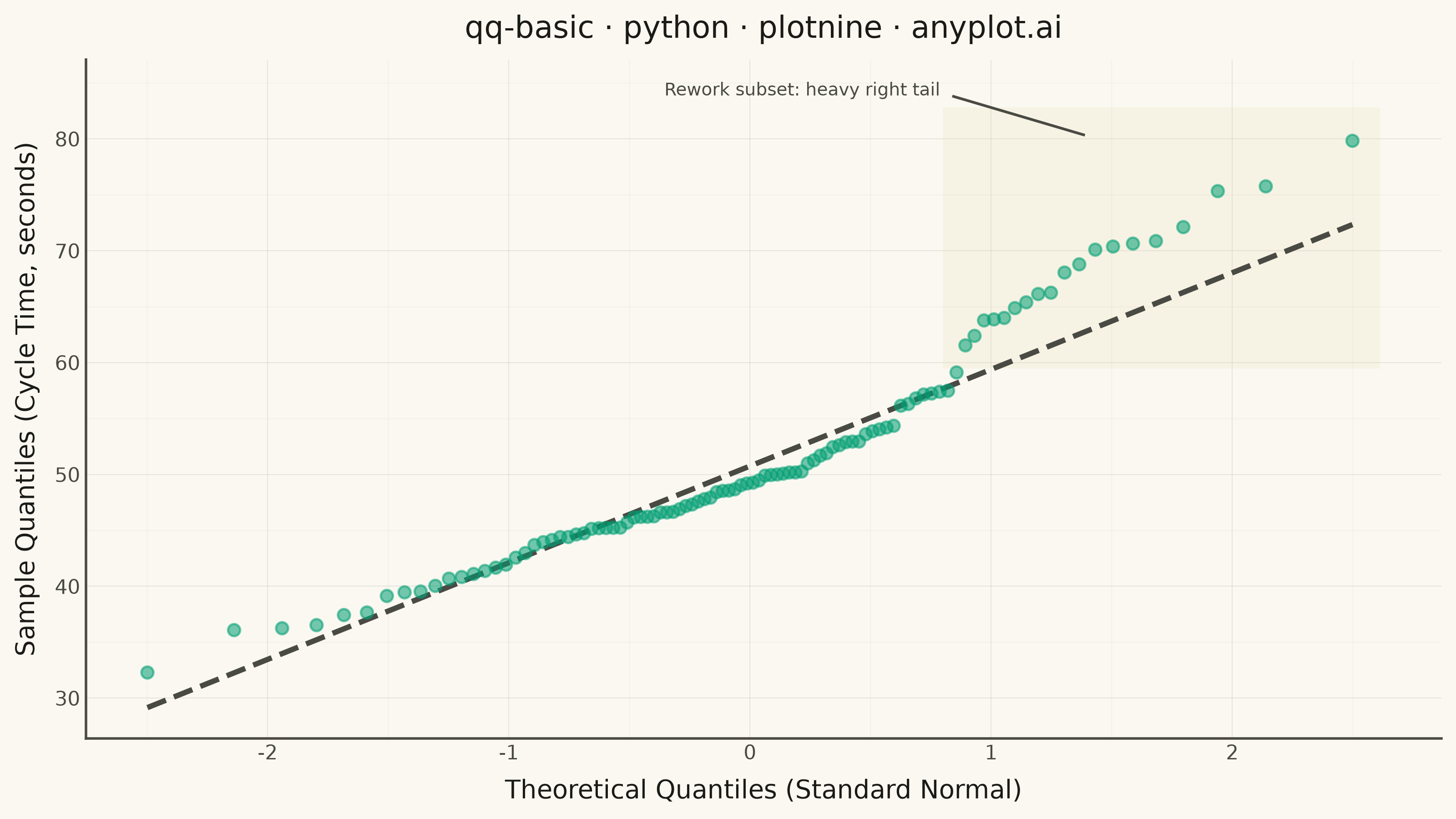
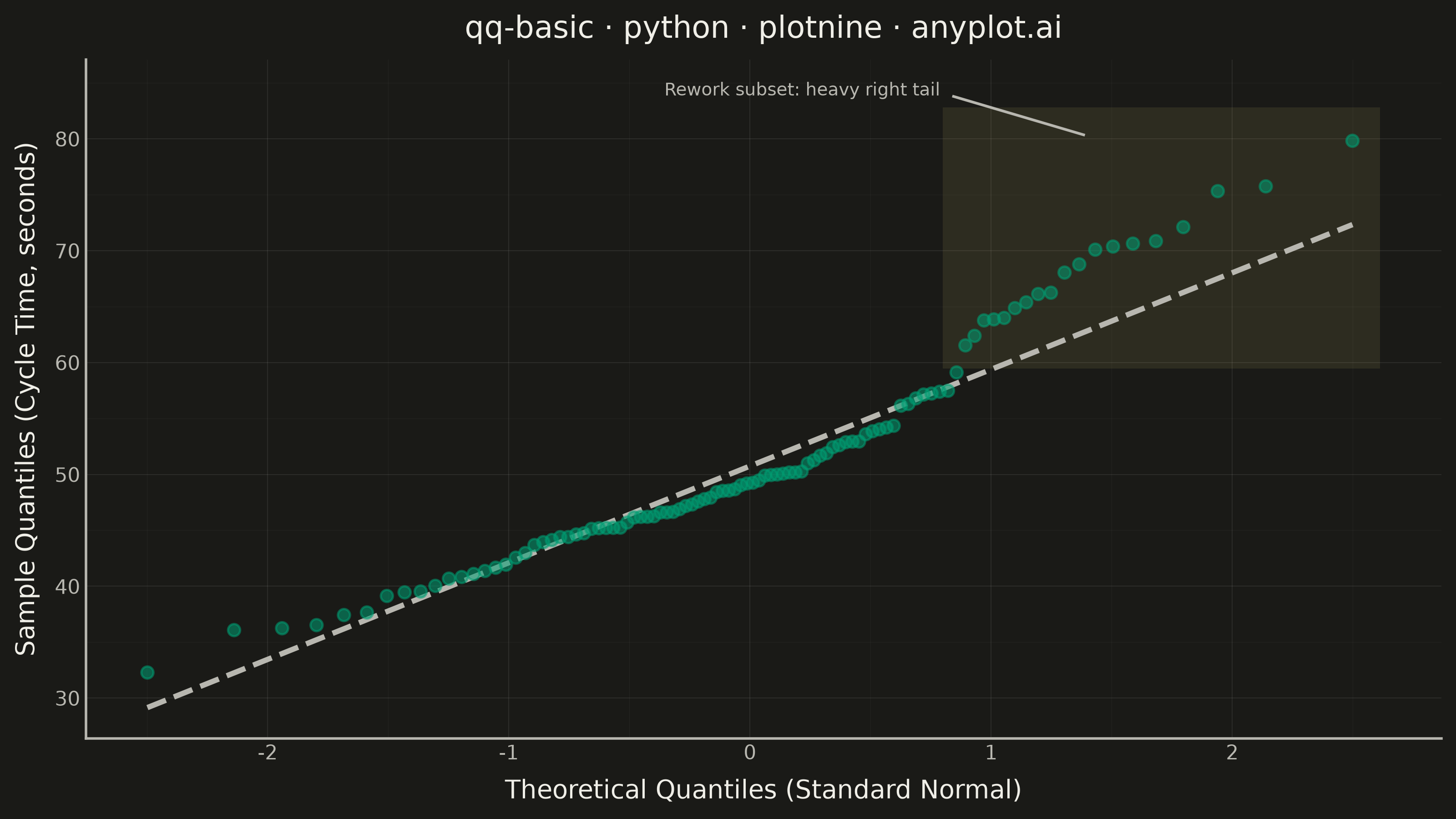
A Q-Q (Quantile-Quantile) plot compares the distribution of a dataset against a theoretical distribution (typically normal) or another dataset. Points are plotted by matching sample quantiles to theoretical quantiles, with a diagonal reference line indicating perfect distribution match. Deviations from the line reveal distribution characteristics such as skewness, heavy tails, and outliers.
""" anyplot.ai
qq-basic: Basic Q-Q Plot
Library: plotnine 0.15.7 | Python 3.13.14
Quality: 90/100 | Updated: 2026-07-24
"""

import os
import sys

import numpy as np
import pandas as pd


# Avoid shadowing the plotnine library when this file is run directly
_cwd = os.getcwd()
sys.path = [p for p in sys.path if os.path.abspath(p) != _cwd]

from plotnine import (
    aes,
    annotate,
    element_line,
    element_rect,
    element_text,
    ggplot,
    labs,
    stat_qq,
    stat_qq_line,
    theme,
    theme_minimal,
)
from scipy import stats


# Theme tokens (Imprint palette)
THEME = os.getenv("ANYPLOT_THEME", "light")
PAGE_BG = "#FAF8F1" if THEME == "light" else "#1A1A17"
INK = "#1A1A17" if THEME == "light" else "#F0EFE8"
INK_SOFT = "#4A4A44" if THEME == "light" else "#B8B7B0"
BRAND = "#009E73"
AMBER = "#DDCC77"

# Data - assembly-line cycle times (seconds). Most parts finish near the
# 48s target, but a rework subset (equipment slowdown / re-machining) runs
# slower, producing a heavy right tail that departs from the normality a
# Six Sigma control chart would otherwise assume.
np.random.seed(42)
cycle_time = np.concatenate([np.random.randn(80) * 6 + 48, np.random.randn(20) * 8 + 68])
df = pd.DataFrame({"cycle_time": cycle_time})

# Locate the tail-departure cluster (for the callout) using the same
# plotting-position convention as stat_qq/stat_qq_line
(theo_q, samp_q), (slope, intercept, _r) = stats.probplot(cycle_time, dist="norm")
fitted = slope * theo_q + intercept
tail_mask = (theo_q > 0.8) & (samp_q - fitted > (samp_q - fitted).std())
callout_x = theo_q[tail_mask].mean()
callout_y = samp_q[tail_mask].max()

plot = (
    ggplot(df, aes(sample="cycle_time"))
    + annotate(
        "rect",
        xmin=0.8,
        xmax=theo_q.max() + 0.15,
        ymin=fitted[theo_q > 0.8].min(),
        ymax=samp_q.max() + 3,
        fill=AMBER,
        alpha=0.10,
    )
    + stat_qq_line(color=INK_SOFT, size=1.2, linetype="dashed")
    + stat_qq(color=BRAND, alpha=0.55, size=2.2)
    + annotate(
        "segment",
        x=callout_x - 0.65,
        y=callout_y + 4,
        xend=callout_x - 0.1,
        yend=callout_y + 0.5,
        color=INK_SOFT,
        size=0.6,
    )
    + annotate(
        "text",
        x=callout_x - 0.7,
        y=callout_y + 4.5,
        label="Rework subset: heavy right tail",
        color=INK_SOFT,
        size=7,
        ha="right",
    )
    + labs(
        x="Theoretical Quantiles (Standard Normal)",
        y="Sample Quantiles (Cycle Time, seconds)",
        title="qq-basic · python · plotnine · anyplot.ai",
    )
    + theme_minimal()
    + theme(
        figure_size=(8, 4.5),
        plot_background=element_rect(fill=PAGE_BG, color=PAGE_BG),
        panel_background=element_rect(fill=PAGE_BG),
        panel_grid_major=element_line(color=INK, size=0.3, alpha=0.10),
        panel_grid_minor=element_line(color=INK, size=0.2, alpha=0.05),
        axis_title=element_text(color=INK, size=10),
        axis_text=element_text(color=INK_SOFT, size=8),
        plot_title=element_text(color=INK, size=12),
        axis_line=element_line(color=INK_SOFT),
    )
)

# Save
plot.save(f"plot-{THEME}.png", dpi=400, width=8, height=4.5, units="in", verbose=False)
Runnable source as JSON, for any HTTP client: https://api.anyplot.ai/specs/qq-basic/plotnine/code. Any spec id and library id listed in llms-full.txt fit the same URL shape; every URL below is complete and callable.
{
  "spec_id": "qq-basic",
  "language": "python",
  "library": "plotnine",
  "page": "https://anyplot.ai/qq-basic/python/plotnine",
  "hub": "https://anyplot.ai/qq-basic",
  "code_json": "https://api.anyplot.ai/specs/qq-basic/plotnine/code",
  "spec_json": "https://api.anyplot.ai/specs/qq-basic",
  "render_light_png": "https://storage.googleapis.com/anyplot-images/plots/qq-basic/python/plotnine/plot-light.png",
  "render_dark_png": "https://storage.googleapis.com/anyplot-images/plots/qq-basic/python/plotnine/plot-dark.png",
  "quality_score": 90.0,
  "license": "MIT",
  "guide": "https://anyplot.ai/llms.txt"
}
Part of Basic Q-Q Plot on anyplot.ai.