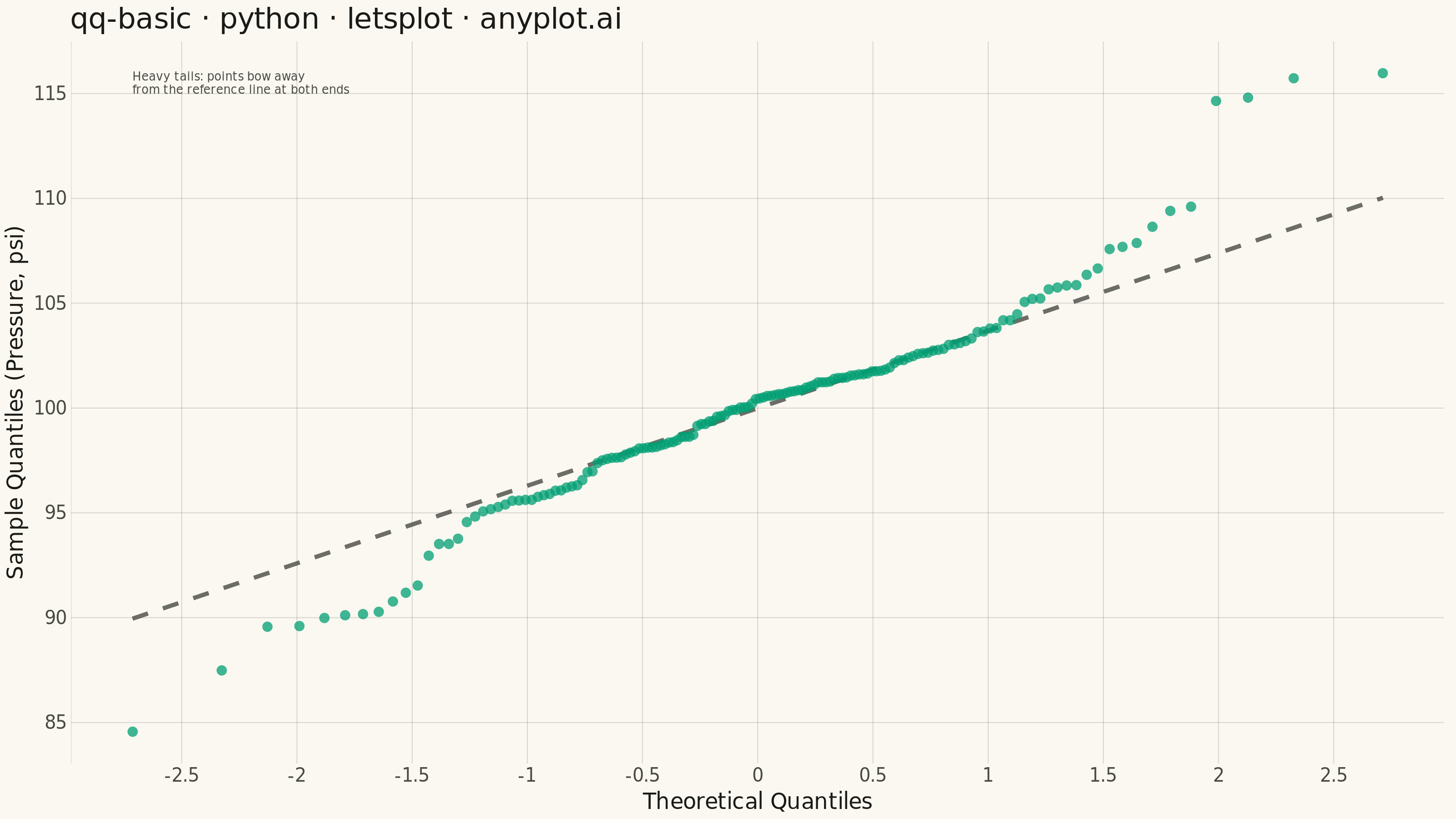
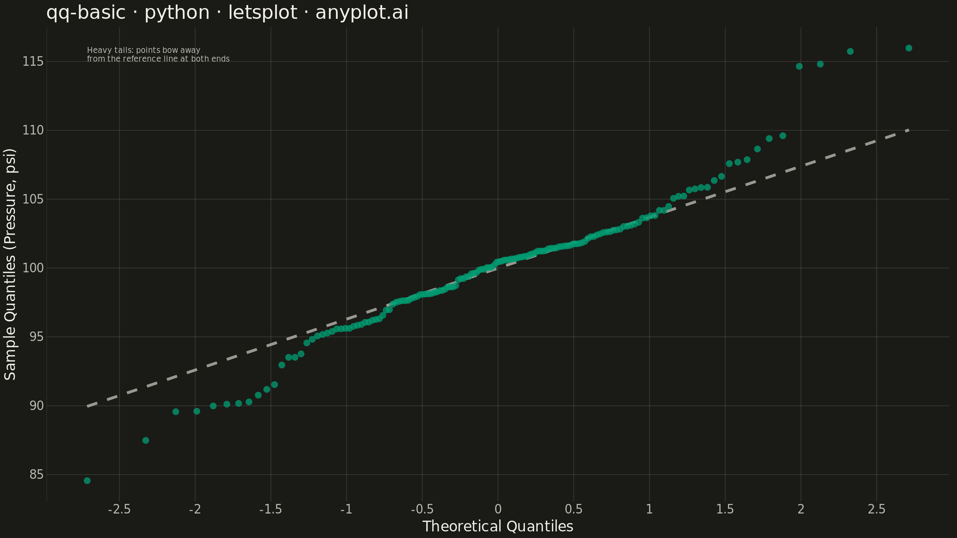
A Q-Q (Quantile-Quantile) plot compares the distribution of a dataset against a theoretical distribution (typically normal) or another dataset. Points are plotted by matching sample quantiles to theoretical quantiles, with a diagonal reference line indicating perfect distribution match. Deviations from the line reveal distribution characteristics such as skewness, heavy tails, and outliers.
""" anyplot.ai
qq-basic: Basic Q-Q Plot
Library: letsplot 4.11.0 | Python 3.13.14
Quality: 91/100 | Updated: 2026-07-24
"""

import os

import numpy as np
import pandas as pd
from lets_plot import (
    LetsPlot,
    aes,
    element_blank,
    element_line,
    element_rect,
    element_text,
    geom_qq,
    geom_qq_line,
    geom_text,
    ggplot,
    ggsize,
    labs,
    theme,
    theme_minimal,
)
from lets_plot.export import ggsave
from scipy import stats


LetsPlot.setup_html()

# Theme tokens (see prompts/default-style-guide.md "Theme-adaptive Chrome")
THEME = os.getenv("ANYPLOT_THEME", "light")
PAGE_BG = "#FAF8F1" if THEME == "light" else "#1A1A17"
INK = "#1A1A17" if THEME == "light" else "#F0EFE8"
INK_SOFT = "#4A4A44" if THEME == "light" else "#B8B7B0"
RULE = "rgba(26,26,23,0.15)" if THEME == "light" else "rgba(240,239,232,0.15)"
BRAND = "#009E73"  # Imprint palette position 1

# Data - pressure readings from a manufacturing QC calibration line, heavy-tailed
# (Student's t, df=3) so both ends of the Q-Q plot bow away from the reference
# line, the classic heavy-tail signature distinct from a simple skew
np.random.seed(42)
pressure_psi = stats.t.rvs(df=3, size=150) * 4 + 100
readings = pd.DataFrame({"pressure_psi": pressure_psi})

# Callout anchored to the sample's own quantile range so it always lands in
# the empty upper-left corner, calling out the story the data was built to tell
n = len(pressure_psi)
callout = pd.DataFrame(
    {
        "x": [stats.norm.ppf(0.5 / n)],
        "y": [readings["pressure_psi"].max()],
        "label": ["Heavy tails: points bow away\nfrom the reference line at both ends"],
    }
)

# Plot - lets-plot's geom_qq/geom_qq_line compute theoretical quantiles and
# the fitted reference line internally against the standard normal. The
# reference line is dashed and muted so the sample points read as the primary
# layer, with the fitted line as a secondary guide.
anyplot_theme = theme(
    plot_background=element_rect(fill=PAGE_BG, color=PAGE_BG),
    panel_background=element_rect(fill=PAGE_BG, color=PAGE_BG),
    panel_border=element_blank(),
    panel_grid_major=element_line(color=RULE, size=0.5),
    panel_grid_minor=element_blank(),
    axis_title=element_text(color=INK, size=12),
    axis_text=element_text(color=INK_SOFT, size=10),
    axis_line=element_line(color=INK_SOFT),
    plot_title=element_text(color=INK, size=16),
)

plot = (
    ggplot(readings, aes(sample="pressure_psi"))
    + geom_qq_line(color=INK_SOFT, size=1.0, linetype="dashed", alpha=0.8)
    + geom_qq(color=BRAND, size=2.5, alpha=0.75)
    + geom_text(
        aes(x="x", y="y", label="label"), data=callout, color=INK_SOFT, size=3.2, hjust=0, vjust=1, lineheight=1.2
    )
    + labs(
        x="Theoretical Quantiles",
        y="Sample Quantiles (Pressure, psi)",
        title="qq-basic · python · letsplot · anyplot.ai",
    )
    + ggsize(800, 450)
    + theme_minimal()
    + anyplot_theme
)

# Save PNG (scale 4x to get 3200 x 1800 px)
ggsave(plot, f"plot-{THEME}.png", path=".", scale=4)

# Save HTML
ggsave(plot, f"plot-{THEME}.html", path=".")
Runnable source as JSON, for any HTTP client: https://api.anyplot.ai/specs/qq-basic/letsplot/code. Any spec id and library id listed in llms-full.txt fit the same URL shape; every URL below is complete and callable.
{
  "spec_id": "qq-basic",
  "language": "python",
  "library": "letsplot",
  "page": "https://anyplot.ai/qq-basic/python/letsplot",
  "hub": "https://anyplot.ai/qq-basic",
  "code_json": "https://api.anyplot.ai/specs/qq-basic/letsplot/code",
  "spec_json": "https://api.anyplot.ai/specs/qq-basic",
  "render_light_png": "https://storage.googleapis.com/anyplot-images/plots/qq-basic/python/letsplot/plot-light.png",
  "render_dark_png": "https://storage.googleapis.com/anyplot-images/plots/qq-basic/python/letsplot/plot-dark.png",
  "interactive_light_html": "https://storage.googleapis.com/anyplot-images/plots/qq-basic/python/letsplot/plot-light.html",
  "interactive_dark_html": "https://storage.googleapis.com/anyplot-images/plots/qq-basic/python/letsplot/plot-dark.html",
  "quality_score": 91.0,
  "license": "MIT",
  "guide": "https://anyplot.ai/llms.txt"
}
Part of Basic Q-Q Plot on anyplot.ai.