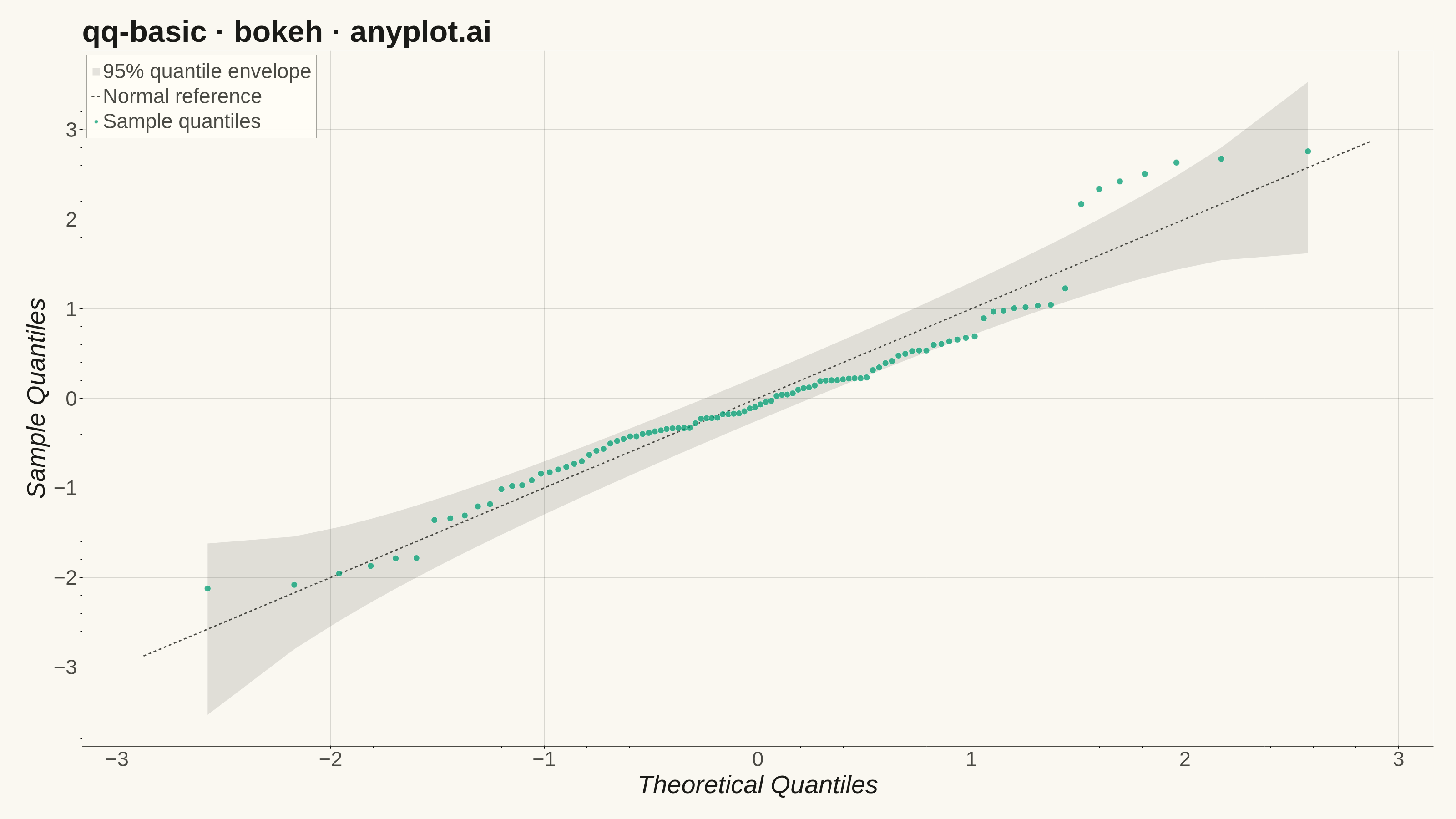
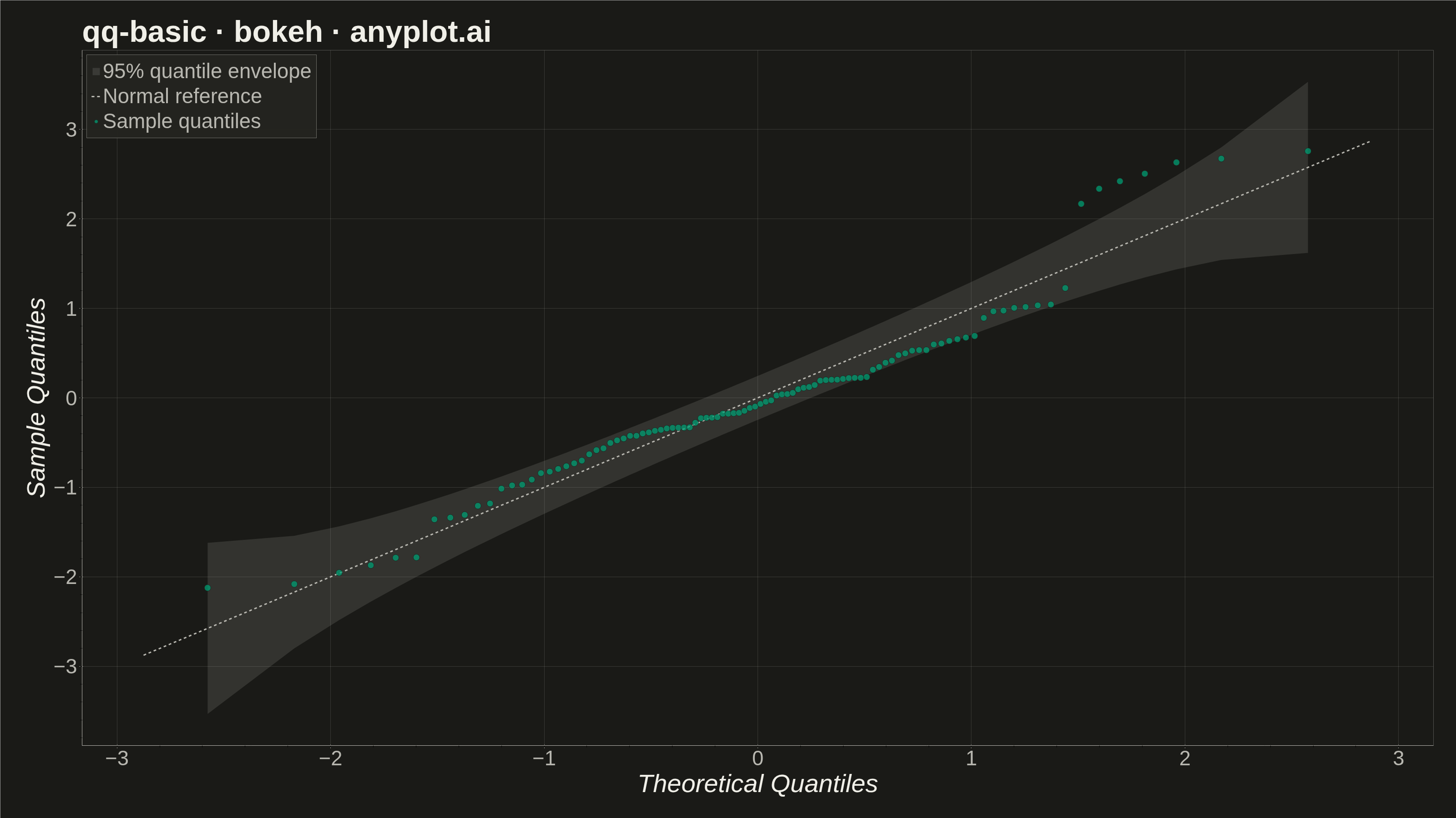
A Q-Q (Quantile-Quantile) plot compares the distribution of a dataset against a theoretical distribution (typically normal) or another dataset. Points are plotted by matching sample quantiles to theoretical quantiles, with a diagonal reference line indicating perfect distribution match. Deviations from the line reveal distribution characteristics such as skewness, heavy tails, and outliers.
""" anyplot.ai
qq-basic: Basic Q-Q Plot
Library: bokeh 3.9.1 | Python 3.13.14
Quality: 90/100 | Updated: 2026-07-24
"""

import io
import os
import time
from pathlib import Path

import numpy as np
from bokeh.io import output_file, save
from bokeh.models import ColumnDataSource, HoverTool
from bokeh.plotting import figure
from PIL import Image
from scipy import stats
from selenium import webdriver
from selenium.webdriver.chrome.options import Options


# Theme tokens (Imprint palette)
THEME = os.getenv("ANYPLOT_THEME", "light")
PAGE_BG = "#FAF8F1" if THEME == "light" else "#1A1A17"
ELEVATED_BG = "#FFFDF6" if THEME == "light" else "#242420"
INK = "#1A1A17" if THEME == "light" else "#F0EFE8"
INK_SOFT = "#4A4A44" if THEME == "light" else "#B8B7B0"
INK_MUTED = "#6B6A63" if THEME == "light" else "#A8A79F"
BRAND = "#009E73"  # Imprint palette position 1

# Data - adult heights (cm) with a few outliers to showcase Q-Q interpretation
np.random.seed(42)
core = np.random.normal(loc=170, scale=8, size=88)
outliers = np.array([145.0, 147.0, 149.0, 196.0, 199.0, 202.0, 148.0, 198.0, 200.0, 203.0, 145.5, 201.5])
sample = np.concatenate([core, outliers])

# Theoretical and sample quantiles (standardised to z-scores)
sample_sorted = np.sort(sample)
n = len(sample_sorted)
probabilities = (np.arange(1, n + 1) - 0.5) / n
theoretical_quantiles = stats.norm.ppf(probabilities)

sample_mean = np.mean(sample)
sample_std = np.std(sample, ddof=1)
sample_quantiles = (sample_sorted - sample_mean) / sample_std

source = ColumnDataSource(
    data={"theoretical": theoretical_quantiles, "sample": sample_quantiles, "value": sample_sorted}
)

# Pointwise 95% confidence envelope for the reference line (order-statistic SE,
# same construction as R's car::qqPlot). It narrows near the median and widens
# in the tails, giving a principled visual cue for which points genuinely
# deviate from normality rather than relying on a text callout.
quantile_se = np.sqrt(probabilities * (1 - probabilities) / n) / stats.norm.pdf(theoretical_quantiles)
z_crit = 1.96
envelope_source = ColumnDataSource(
    data={
        "base": theoretical_quantiles,
        "lower": theoretical_quantiles - z_crit * quantile_se,
        "upper": theoretical_quantiles + z_crit * quantile_se,
    }
)

# Reference line (y=x, bounded to data range)
pad = 0.3
x_min = theoretical_quantiles.min() - pad
x_max = theoretical_quantiles.max() + pad

# Figure — canvas is a hard 3200x1800 contract; min_border_* reserve room for
# the 42pt axis labels + 34pt tick labels so they aren't clipped from the PNG.
p = figure(
    width=3200,
    height=1800,
    title="qq-basic · bokeh · anyplot.ai",
    x_axis_label="Theoretical Quantiles",
    y_axis_label="Sample Quantiles",
    toolbar_location=None,
    min_border_bottom=160,
    min_border_left=180,
    min_border_top=110,
    min_border_right=50,
)

# Confidence envelope drawn first so the line and points sit on top of it
p.varea(
    x="base",
    y1="lower",
    y2="upper",
    source=envelope_source,
    fill_color=INK_MUTED,
    fill_alpha=0.18,
    legend_label="95% quantile envelope",
)

# Reference line drawn as a line glyph so it can carry a legend label
p.line(
    [x_min, x_max],
    [x_min, x_max],
    line_color=INK_SOFT,
    line_width=3,
    line_dash="dashed",
    legend_label="Normal reference",
)

# Q-Q scatter points
p.scatter(
    x="theoretical",
    y="sample",
    source=source,
    size=14,
    color=BRAND,
    alpha=0.75,
    line_color=PAGE_BG,
    line_width=1,
    legend_label="Sample quantiles",
)

# Hover tooltips
hover = HoverTool(
    tooltips=[("Theoretical Q", "@theoretical{0.00}"), ("Sample Q", "@sample{0.00}"), ("Height", "@value{0.0} cm")]
)
p.add_tools(hover)

# Theme-adaptive chrome
p.background_fill_color = PAGE_BG
p.border_fill_color = PAGE_BG
p.outline_line_color = None  # drop the boxed-in frame; left/bottom axis lines are enough

p.title.text_color = INK
p.title.text_font_size = "50pt"

p.xaxis.axis_label_text_color = INK
p.yaxis.axis_label_text_color = INK
p.xaxis.axis_label_text_font_size = "42pt"
p.yaxis.axis_label_text_font_size = "42pt"
p.xaxis.major_label_text_color = INK_SOFT
p.yaxis.major_label_text_color = INK_SOFT
p.xaxis.major_label_text_font_size = "34pt"
p.yaxis.major_label_text_font_size = "34pt"
p.xaxis.axis_line_color = INK_SOFT
p.yaxis.axis_line_color = INK_SOFT
p.xaxis.major_tick_line_color = INK_SOFT
p.yaxis.major_tick_line_color = INK_SOFT

p.xgrid.grid_line_color = INK
p.ygrid.grid_line_color = INK
p.xgrid.grid_line_alpha = 0.15
p.ygrid.grid_line_alpha = 0.15

if p.legend:
    p.legend.background_fill_color = ELEVATED_BG
    p.legend.border_line_color = INK_SOFT
    p.legend.label_text_color = INK_SOFT
    p.legend.label_text_font_size = "34pt"
    p.legend.location = "top_left"
    p.legend.click_policy = "hide"  # toggle envelope / reference / points

# Save HTML (interactive artifact) and screenshot it with headless Chrome.
# bokeh.io.export_png is avoided: it probes /usr/bin/chromedriver, which is a
# snap shim on this box and fails regardless of xvfb — Selenium's own driver
# resolution (Selenium Manager) works instead.
output_file(f"plot-{THEME}.html")
save(p)

# Window is H+200 tall so the browser chrome (present even headless) doesn't
# eat into the bokeh canvas; PIL crops the screenshot back to exactly W x H.
W, H = 3200, 1800
opts = Options()
for arg in (
    "--headless=new",
    "--no-sandbox",
    "--disable-dev-shm-usage",
    "--disable-gpu",
    f"--window-size={W},{H + 200}",
    "--hide-scrollbars",
    "--force-device-scale-factor=1",
):
    opts.add_argument(arg)
driver = webdriver.Chrome(options=opts)
driver.set_window_size(W, H + 200)
driver.get(f"file://{Path(f'plot-{THEME}.html').resolve()}")
time.sleep(3)  # let bokeh's JS render the canvas
raw = driver.get_screenshot_as_png()
driver.quit()
Image.open(io.BytesIO(raw)).crop((0, 0, W, H)).save(f"plot-{THEME}.png")
Runnable source as JSON, for any HTTP client: https://api.anyplot.ai/specs/qq-basic/bokeh/code. Any spec id and library id listed in llms-full.txt fit the same URL shape; every URL below is complete and callable.
{
  "spec_id": "qq-basic",
  "language": "python",
  "library": "bokeh",
  "page": "https://anyplot.ai/qq-basic/python/bokeh",
  "hub": "https://anyplot.ai/qq-basic",
  "code_json": "https://api.anyplot.ai/specs/qq-basic/bokeh/code",
  "spec_json": "https://api.anyplot.ai/specs/qq-basic",
  "render_light_png": "https://storage.googleapis.com/anyplot-images/plots/qq-basic/python/bokeh/plot-light.png",
  "render_dark_png": "https://storage.googleapis.com/anyplot-images/plots/qq-basic/python/bokeh/plot-dark.png",
  "interactive_light_html": "https://storage.googleapis.com/anyplot-images/plots/qq-basic/python/bokeh/plot-light.html",
  "interactive_dark_html": "https://storage.googleapis.com/anyplot-images/plots/qq-basic/python/bokeh/plot-dark.html",
  "quality_score": 90.0,
  "license": "MIT",
  "guide": "https://anyplot.ai/llms.txt"
}
Part of Basic Q-Q Plot on anyplot.ai.