The same plot in 14 other libraries — JavaScript: Chart.js, D3.js, Apache ECharts, MUI X Charts; Python: Altair, Bokeh, lets-plot, Matplotlib, Plotly, plotnine, Pygal, Seaborn; R: ggplot2; Julia: Makie.jl. Compare all 15 side by side: Basic Q-Q Plot in Python, R, Julia and JavaScript.
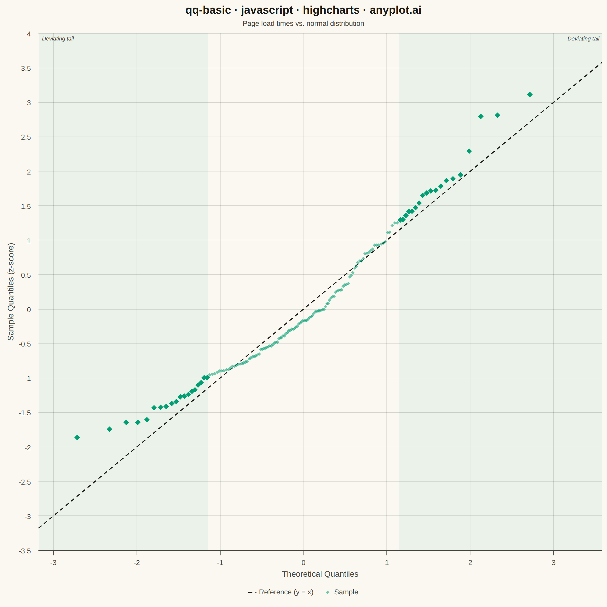
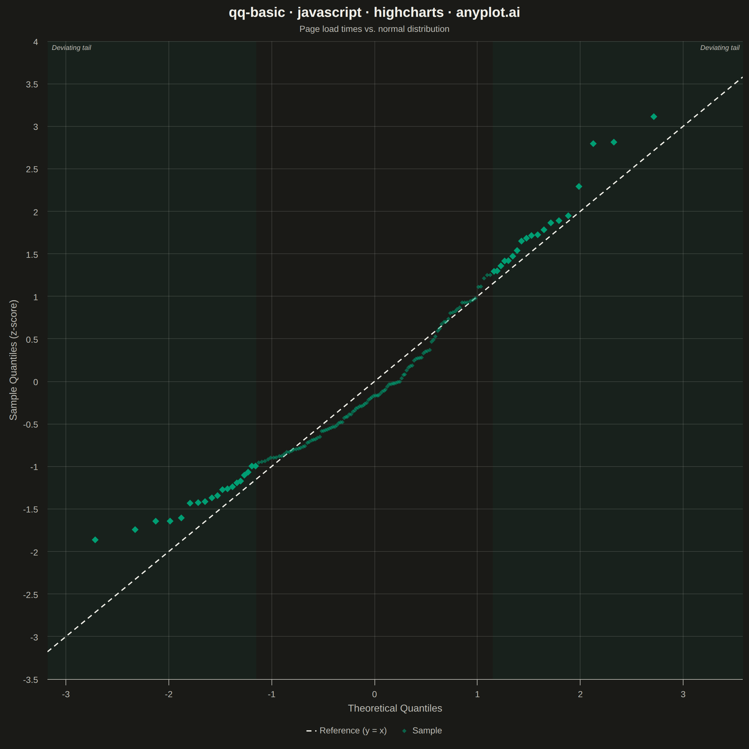
A Q-Q (Quantile-Quantile) plot compares the distribution of a dataset against a theoretical distribution (typically normal) or another dataset. Points are plotted by matching sample quantiles to theoretical quantiles, with a reference line indicating perfect distribution match. Deviations from the line reveal distribution characteristics such as skewness, heavy tails, and outliers.
// anyplot.ai
// qq-basic: Basic Q-Q Plot
// Library: highcharts 12.6.0 | JavaScript 22.23.1
// Quality: 92/100 | Created: 2026-07-24

//# anyplot-orientation: square
const t = window.ANYPLOT_TOKENS;

// --- Data (in-memory, deterministic) ----------------------------------------
// Website page-load times: right-skewed (lognormal-ish), a classic case where
// a normality assumption needs checking before applying parametric tests.
function lcg(seed) {
  let state = seed;
  return function () {
    state = (state * 1664525 + 1013904223) % 4294967296;
    return state / 4294967296;
  };
}
const rand = lcg(42);

function randNormal() {
  const u1 = Math.max(rand(), 1e-9);
  const u2 = rand();
  return Math.sqrt(-2 * Math.log(u1)) * Math.cos(2 * Math.PI * u2);
}

// Inverse standard normal CDF (Acklam's rational approximation).
function invNorm(p) {
  const a = [-3.969683028665376e1, 2.209460984245205e2, -2.759285104469687e2,
             1.383577518672690e2, -3.066479806614716e1, 2.506628277459239e0];
  const b = [-5.447609879822406e1, 1.615858368580409e2, -1.556989798598866e2,
             6.680131188771972e1, -1.328068155288572e1];
  const c = [-7.784894002430293e-3, -3.223964580411365e-1, -2.400758277161838e0,
             -2.549732539343734e0, 4.374664141464968e0, 2.938163982698783e0];
  const d = [7.784695709041462e-3, 3.224671290700398e-1, 2.445134137142996e0,
             3.754408661907416e0];
  const pLow = 0.02425;
  const pHigh = 1 - pLow;
  if (p < pLow) {
    const q = Math.sqrt(-2 * Math.log(p));
    return (((((c[0] * q + c[1]) * q + c[2]) * q + c[3]) * q + c[4]) * q + c[5]) /
           ((((d[0] * q + d[1]) * q + d[2]) * q + d[3]) * q + 1);
  }
  if (p <= pHigh) {
    const q = p - 0.5;
    const r = q * q;
    return (((((a[0] * r + a[1]) * r + a[2]) * r + a[3]) * r + a[4]) * r + a[5]) * q /
           (((((b[0] * r + b[1]) * r + b[2]) * r + b[3]) * r + b[4]) * r + 1);
  }
  const q = Math.sqrt(-2 * Math.log(1 - p));
  return -(((((c[0] * q + c[1]) * q + c[2]) * q + c[3]) * q + c[4]) * q + c[5]) /
          ((((d[0] * q + d[1]) * q + d[2]) * q + d[3]) * q + 1);
}

const n = 150;
const muLog = -0.35;
const sigmaLog = 0.45;
const loadTimes = [];
for (let i = 0; i < n; i++) {
  loadTimes.push(Math.exp(muLog + sigmaLog * randNormal()));
}
loadTimes.sort((a, b) => a - b);

const mean = loadTimes.reduce((s, v) => s + v, 0) / n;
const variance = loadTimes.reduce((s, v) => s + (v - mean) ** 2, 0) / (n - 1);
const std = Math.sqrt(variance);

// Standardized sample quantiles vs. theoretical normal quantiles — under a
// perfect normal fit, points fall on the y = x diagonal.
const points = loadTimes.map((value, i) => {
  const p = (i + 0.5) / n;
  const theoreticalQ = invNorm(p);
  const sampleQ = (value - mean) / std;
  return [theoreticalQ, sampleQ];
});

const allValues = points.flat();
const lo = Math.min(...allValues);
const hi = Math.max(...allValues);
const pad = (hi - lo) * 0.08;
const axisMin = lo - pad;
const axisMax = hi + pad;

// Points beyond this theoretical quantile are the "tail" where the sample
// visibly bows away from the reference line. They get a larger, fully-opaque
// marker; the tightly-packed mid-section gets a smaller, translucent one so
// the S-curve deviation reads clearly instead of the middle overlapping.
const tailThreshold = 1.15;
function withAlpha(hex, alpha) {
  const r = parseInt(hex.slice(1, 3), 16);
  const g = parseInt(hex.slice(3, 5), 16);
  const b = parseInt(hex.slice(5, 7), 16);
  return `rgba(${r}, ${g}, ${b}, ${alpha})`;
}
const sampleColor = t.palette[0];
const midColor = withAlpha(sampleColor, 0.55);
const scatterData = points.map(([x, y]) => ({
  x,
  y,
  marker: Math.abs(x) > tailThreshold
    ? { radius: 5.5, fillColor: sampleColor }
    : { radius: 3.5, fillColor: midColor },
}));

// --- Chart -------------------------------------------------------------------
Highcharts.chart("container", {
  chart: { type: "scatter", backgroundColor: "transparent", animation: false,
           style: { fontFamily: "inherit" } },
  credits: { enabled: false },
  colors: t.palette,
  title: { text: "qq-basic · javascript · highcharts · anyplot.ai",
           style: { color: t.ink, fontSize: "22px", fontWeight: "600" } },
  subtitle: { text: "Page load times vs. normal distribution",
              style: { color: t.inkSoft, fontSize: "14px" } },
  xAxis: { title: { text: "Theoretical Quantiles",
                     style: { color: t.inkSoft, fontSize: "16px" } },
           min: axisMin, max: axisMax,
           lineColor: t.inkSoft, tickColor: t.inkSoft, gridLineColor: t.grid,
           gridLineWidth: 1,
           labels: { style: { color: t.inkSoft, fontSize: "14px" } },
           plotBands: [
             { from: axisMin, to: -tailThreshold, color: withAlpha(sampleColor, 0.06),
               label: { text: "Deviating tail", align: "left", x: 6, y: 14,
                        style: { color: t.inkSoft, fontSize: "11px", fontStyle: "italic" } } },
             { from: tailThreshold, to: axisMax, color: withAlpha(sampleColor, 0.06),
               label: { text: "Deviating tail", align: "right", x: -6, y: 14,
                        style: { color: t.inkSoft, fontSize: "11px", fontStyle: "italic" } } },
           ] },
  yAxis: { title: { text: "Sample Quantiles (z-score)",
                     style: { color: t.inkSoft, fontSize: "16px" } },
           min: axisMin, max: axisMax,
           lineColor: t.inkSoft, tickColor: t.inkSoft, gridLineColor: t.grid,
           labels: { style: { color: t.inkSoft, fontSize: "14px" } } },
  legend: { itemStyle: { color: t.inkSoft, fontSize: "14px" },
            itemHoverStyle: { color: t.ink } },
  plotOptions: { series: { animation: false } },
  series: [
    {
      name: "Reference (y = x)",
      type: "line",
      data: [[axisMin, axisMin], [axisMax, axisMax]],
      color: t.ink,
      dashStyle: "Dash",
      lineWidth: 2,
      marker: { enabled: false },
      enableMouseTracking: false,
    },
    {
      name: "Sample",
      type: "scatter",
      data: scatterData,
      color: sampleColor,
      marker: { radius: 3.5, fillColor: midColor },
    },
  ],
});
Runnable source as JSON, for any HTTP client: https://api.anyplot.ai/specs/qq-basic/highcharts/code. Any spec id and library id listed in llms-full.txt fit the same URL shape; every URL below is complete and callable.
{
  "spec_id": "qq-basic",
  "language": "javascript",
  "library": "highcharts",
  "page": "https://anyplot.ai/qq-basic/javascript/highcharts",
  "hub": "https://anyplot.ai/qq-basic",
  "code_json": "https://api.anyplot.ai/specs/qq-basic/highcharts/code",
  "spec_json": "https://api.anyplot.ai/specs/qq-basic",
  "render_light_png": "https://storage.googleapis.com/anyplot-images/plots/qq-basic/javascript/highcharts/plot-light.png",
  "render_dark_png": "https://storage.googleapis.com/anyplot-images/plots/qq-basic/javascript/highcharts/plot-dark.png",
  "interactive_light_html": "https://storage.googleapis.com/anyplot-images/plots/qq-basic/javascript/highcharts/plot-light.html",
  "interactive_dark_html": "https://storage.googleapis.com/anyplot-images/plots/qq-basic/javascript/highcharts/plot-dark.html",
  "quality_score": 92.0,
  "license": "MIT",
  "guide": "https://anyplot.ai/llms.txt"
}
Part of Basic Q-Q Plot on anyplot.ai.