The same plot in 14 other libraries — JavaScript: D3.js, Apache ECharts, Highcharts, MUI X Charts; Python: Altair, Bokeh, lets-plot, Matplotlib, Plotly, plotnine, Pygal, Seaborn; R: ggplot2; Julia: Makie.jl. Compare all 15 side by side: Residual Plot in Python, R, Julia and JavaScript.
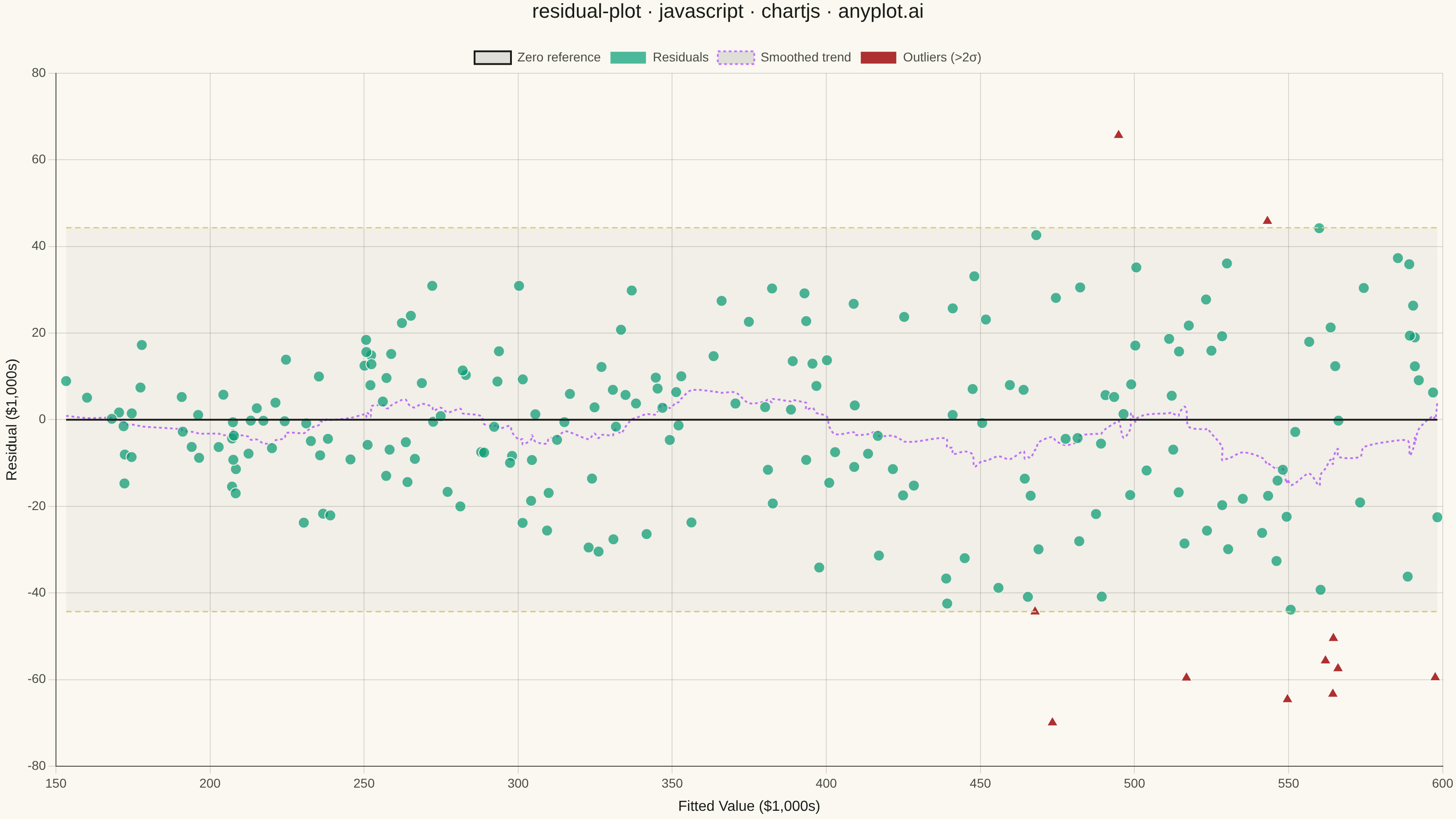
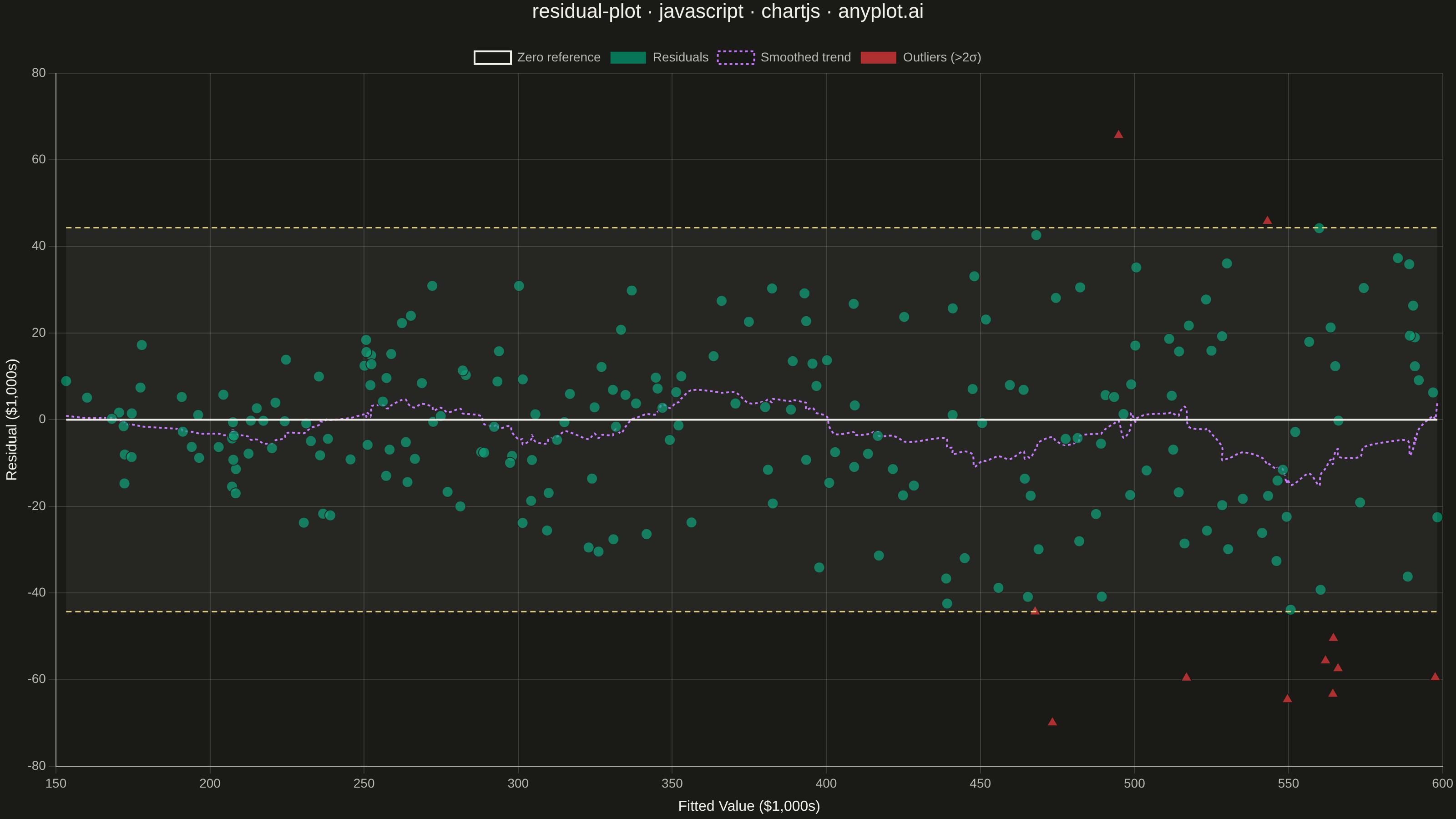
A residual plot displays the difference between observed and predicted values (residuals) against fitted values in regression analysis. This diagnostic visualization helps identify violations of regression assumptions including non-linearity, heteroscedasticity (non-constant variance), and outliers. A well-fitting model shows residuals randomly scattered around zero with no discernible pattern.
// anyplot.ai
// residual-plot: Residual Plot
// Library: chartjs 4.4.7 | JavaScript 22.23.2
// Quality: 94/100 | Created: 2026-09-05

const t = window.ANYPLOT_TOKENS;

// --- Data (in-memory, deterministic LCG) ------------------------------------
// Simulated linear-regression diagnostics: fitted house-price predictions
// (in $1000s) vs. residuals, with mild heteroscedasticity (variance grows
// with fitted value) so the fan-out pattern is visible.
let seed = 42;
function lcg() {
  seed = (seed * 1664525 + 1013904223) % 4294967296;
  return seed / 4294967296;
}
function gaussian() {
  const u1 = 1 - lcg();
  const u2 = lcg();
  return Math.sqrt(-2 * Math.log(u1)) * Math.cos(2 * Math.PI * u2);
}
function hexToRgba(hex, alpha) {
  const h = hex.replace("#", "");
  const r = parseInt(h.substring(0, 2), 16);
  const g = parseInt(h.substring(2, 4), 16);
  const b = parseInt(h.substring(4, 6), 16);
  return `rgba(${r}, ${g}, ${b}, ${alpha})`;
}

const n = 220;
const fitted = [];
const residuals = [];
for (let i = 0; i < n; i++) {
  const value = 150 + lcg() * 450; // fitted price, $150k-$600k
  const noiseScale = 8 + (value - 150) * 0.05; // heteroscedastic spread
  fitted.push(value);
  residuals.push(gaussian() * noiseScale);
}

const mean = residuals.reduce((a, b) => a + b, 0) / n;
const variance = residuals.reduce((a, b) => a + (b - mean) ** 2, 0) / n;
const stdDev = Math.sqrt(variance);
const threshold = 2 * stdDev;

const normalPoints = [];
const outlierPoints = [];
for (let i = 0; i < n; i++) {
  const point = { x: fitted[i], y: residuals[i] };
  if (Math.abs(residuals[i]) > threshold) {
    outlierPoints.push(point);
  } else {
    normalPoints.push(point);
  }
}

const xMin = Math.min(...fitted);
const xMax = Math.max(...fitted);

// Rolling-mean smoothing trend (sorted by fitted value) to surface any
// residual non-linearity — optional per spec, adds diagnostic value.
const sortedIdx = fitted.map((_, i) => i).sort((a, b) => fitted[a] - fitted[b]);
const sortedX = sortedIdx.map((i) => fitted[i]);
const sortedY = sortedIdx.map((i) => residuals[i]);
const windowSize = Math.max(15, Math.round(n * 0.12));
const trendPoints = sortedX.map((x, i) => {
  const lo = Math.max(0, i - Math.floor(windowSize / 2));
  const hi = Math.min(n, i + Math.ceil(windowSize / 2));
  const slice = sortedY.slice(lo, hi);
  const avg = slice.reduce((a, b) => a + b, 0) / slice.length;
  return { x, y: avg };
});

// --- Mount -------------------------------------------------------------------
const canvas = document.createElement("canvas");
document.getElementById("container").appendChild(canvas);

// --- Chart ---------------------------------------------------------------------
new Chart(canvas, {
  type: "scatter",
  data: {
    datasets: [
      {
        label: "±2σ band",
        data: [
          { x: xMin, y: threshold },
          { x: xMax, y: threshold },
        ],
        showLine: true,
        borderColor: t.amber,
        borderWidth: 1.5,
        borderDash: [6, 4],
        pointRadius: 0,
        fill: "+2",
        backgroundColor:
          t.pageBg === "#1A1A17" ? "rgba(240,239,232,0.06)" : "rgba(26,26,23,0.04)",
      },
      {
        label: "Zero reference",
        data: [
          { x: xMin, y: 0 },
          { x: xMax, y: 0 },
        ],
        showLine: true,
        borderColor: t.ink,
        borderWidth: 2,
        pointRadius: 0,
      },
      {
        label: "−2σ band",
        data: [
          { x: xMin, y: -threshold },
          { x: xMax, y: -threshold },
        ],
        showLine: true,
        borderColor: t.amber,
        borderWidth: 1.5,
        borderDash: [6, 4],
        pointRadius: 0,
      },
      {
        label: "Residuals",
        data: normalPoints,
        backgroundColor: hexToRgba(t.palette[0], 0.7),
        borderColor: t.pageBg,
        borderWidth: 1,
        pointRadius: 6,
        pointHoverRadius: 7,
      },
      {
        label: "Smoothed trend",
        data: trendPoints,
        showLine: true,
        borderColor: t.palette[1],
        borderWidth: 2,
        borderDash: [3, 3],
        pointRadius: 0,
        fill: false,
        tension: 0.3,
      },
      {
        label: "Outliers (>2σ)",
        data: outlierPoints,
        backgroundColor: t.palette[4],
        borderColor: t.pageBg,
        borderWidth: 1,
        pointRadius: 7,
        pointStyle: "triangle",
        pointHoverRadius: 8,
      },
    ],
  },
  options: {
    responsive: true,
    maintainAspectRatio: false,
    animation: false,
    plugins: {
      title: {
        display: true,
        text: "residual-plot · javascript · chartjs · anyplot.ai",
        color: t.ink,
        font: { size: 22, weight: "500" },
        padding: { bottom: 20 },
      },
      legend: {
        labels: {
          color: t.inkSoft,
          font: { size: 14 },
          filter: (item) => item.text !== "±2σ band" && item.text !== "−2σ band",
        },
      },
      tooltip: { enabled: false },
    },
    scales: {
      x: {
        type: "linear",
        title: { display: true, text: "Fitted Value ($1,000s)", color: t.ink, font: { size: 16 } },
        ticks: { color: t.inkSoft, font: { size: 14 } },
        grid: { color: t.grid },
        border: { color: t.inkSoft },
      },
      y: {
        title: { display: true, text: "Residual ($1,000s)", color: t.ink, font: { size: 16 } },
        ticks: { color: t.inkSoft, font: { size: 14 } },
        grid: { color: t.grid },
        border: { color: t.inkSoft },
      },
    },
  },
});
Runnable source as JSON, for any HTTP client: https://api.anyplot.ai/specs/residual-plot/chartjs/code. Any spec id and library id listed in llms-full.txt fit the same URL shape; every URL below is complete and callable.
{
  "spec_id": "residual-plot",
  "language": "javascript",
  "library": "chartjs",
  "page": "https://anyplot.ai/residual-plot/javascript/chartjs",
  "hub": "https://anyplot.ai/residual-plot",
  "code_json": "https://api.anyplot.ai/specs/residual-plot/chartjs/code",
  "spec_json": "https://api.anyplot.ai/specs/residual-plot",
  "render_light_png": "https://storage.googleapis.com/anyplot-images/plots/residual-plot/javascript/chartjs/plot-light.png",
  "render_dark_png": "https://storage.googleapis.com/anyplot-images/plots/residual-plot/javascript/chartjs/plot-dark.png",
  "interactive_light_html": "https://storage.googleapis.com/anyplot-images/plots/residual-plot/javascript/chartjs/plot-light.html",
  "interactive_dark_html": "https://storage.googleapis.com/anyplot-images/plots/residual-plot/javascript/chartjs/plot-dark.html",
  "quality_score": 94.0,
  "license": "MIT",
  "guide": "https://anyplot.ai/llms.txt"
}
Part of Residual Plot on anyplot.ai.