Residual Plot — D3.js

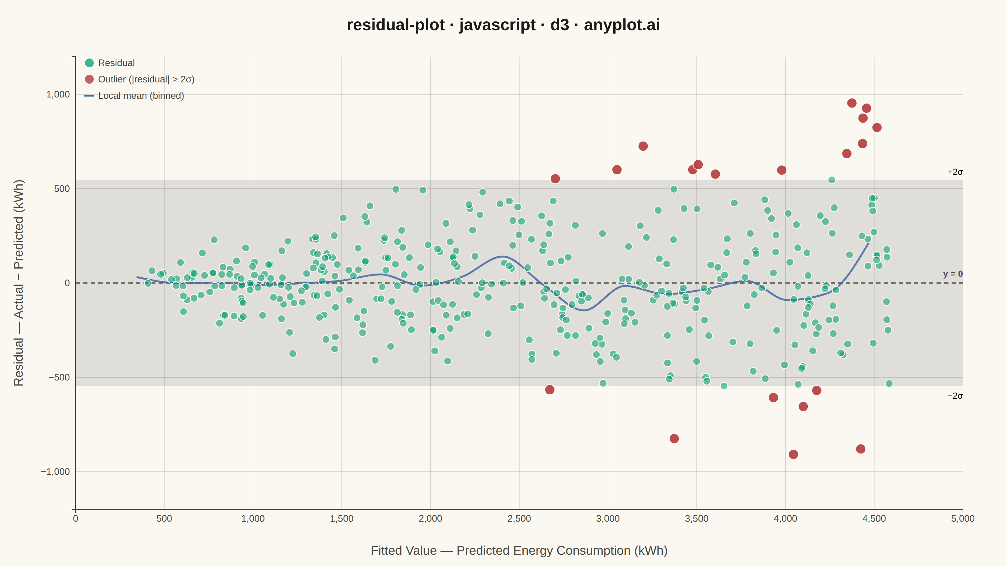
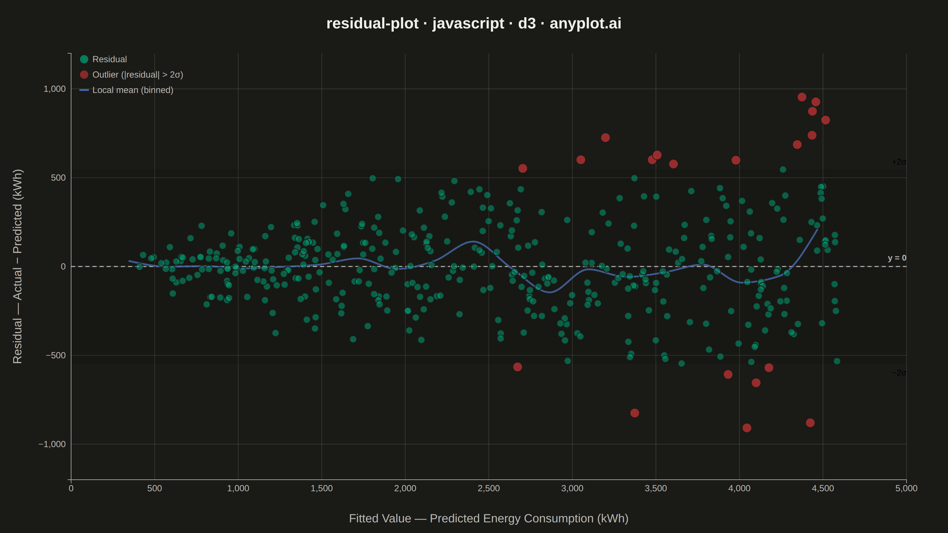
A residual plot displays the difference between observed and predicted values (residuals) against fitted values or an independent variable in regression analysis. This diagnostic visualization helps identify violations of regression assumptions including non-linearity, heteroscedasticity (non-constant variance), and outliers. A well-fitting model shows residuals randomly scattered around zero with no discernible pattern.

Renders

• Full-resolution render, light theme
• Full-resolution render, dark theme
• Interactive version, light theme
• Interactive version, dark theme

JavaScript source (D3.js)

// anyplot.ai
// residual-plot: Residual Plot
// Library: d3 7.9.0 | JavaScript 22.23.2
// Quality: 90/100 | Created: 2026-09-05

const t = window.ANYPLOT_TOKENS;
const { width, height } = window.ANYPLOT_SIZE;
const margin = { top: 90, right: 70, bottom: 90, left: 120 };
const iw = width - margin.left - margin.right;
const ih = height - margin.top - margin.bottom;

// --- Data (deterministic LCG seed=42, building energy-consumption model) ---
let seed = 42;
function lcgRand() {
  seed = (1664525 * seed + 1013904223) >>> 0;
  return seed / 4294967296;
}
function lcgRandn() {
  const u1 = lcgRand() + 1e-10;
  const u2 = lcgRand();
  return Math.sqrt(-2 * Math.log(u1)) * Math.cos(2 * Math.PI * u2);
}

// Predicted monthly energy consumption (kWh) from a regression model, with a
// deliberately heteroscedastic error term — the variance of the residual
// grows with the fitted value, a classic diagnostic finding.
const data = Array.from({ length: 400 }, () => {
  const fitted = 400 + lcgRand() * 4200;
  const noiseScale = 55 + fitted * 0.085;
  const residual = lcgRandn() * noiseScale;
  return { fitted, residual };
});

// --- Reference statistics ---------------------------------------------------
const rmsResidual = Math.sqrt(d3.mean(data, (d) => d.residual ** 2));
const outlierThreshold = 2 * rmsResidual;
data.forEach((d) => {
  d.isOutlier = Math.abs(d.residual) > outlierThreshold;
});

// --- Binned local-mean smoother (LOWESS-style trend of the residual mean) --
const N_BINS = 20;
const fittedMax = d3.max(data, (d) => d.fitted);
const binWidth = fittedMax / N_BINS;
const bins = Array.from({ length: N_BINS }, () => []);
data.forEach((d) => {
  const idx = Math.min(N_BINS - 1, Math.floor(d.fitted / binWidth));
  bins[idx].push(d.residual);
});
const smoothed = bins
  .map((vals, i) => (vals.length ? { fitted: (i + 0.5) * binWidth, residual: d3.mean(vals) } : null))
  .filter((d) => d !== null);

// --- SVG mount ---------------------------------------------------------------
const svg = d3.select("#container").append("svg").attr("width", width).attr("height", height);
const g = svg.append("g").attr("transform", `translate(${margin.left},${margin.top})`);

// --- Scales -------------------------------------------------------------------
const x = d3.scaleLinear().domain([0, fittedMax * 1.03]).nice().range([0, iw]);

const maxAbsResidual = Math.max(d3.max(data, (d) => Math.abs(d.residual)), outlierThreshold) * 1.15;
const y = d3.scaleLinear().domain([-maxAbsResidual, maxAbsResidual]).nice().range([ih, 0]);

// --- Grid (both axes, floating — no domain line, matches scatter convention)
g.append("g")
  .attr("transform", `translate(0,${ih})`)
  .call(d3.axisBottom(x).ticks(8).tickSize(-ih).tickFormat(""))
  .call((ax) => ax.select(".domain").remove())
  .call((ax) => ax.selectAll("line").attr("stroke", t.grid));

g.append("g")
  .call(d3.axisLeft(y).ticks(7).tickSize(-iw).tickFormat(""))
  .call((ax) => ax.select(".domain").remove())
  .call((ax) => ax.selectAll("line").attr("stroke", t.grid));

// --- +/-2 sigma band (muted fill, identifies the potential-outlier zone) ---
g.append("rect")
  .attr("x", 0)
  .attr("y", y(outlierThreshold))
  .attr("width", iw)
  .attr("height", y(-outlierThreshold) - y(outlierThreshold))
  .attr("fill", t.muted)
  .attr("fill-opacity", 0.1);

g.selectAll(".band-line")
  .data([outlierThreshold, -outlierThreshold])
  .join("line")
  .attr("x1", 0).attr("x2", iw)
  .attr("y1", (d) => y(d)).attr("y2", (d) => y(d))
  .attr("stroke", t.muted)
  .attr("stroke-width", 1.5)
  .attr("stroke-dasharray", "3,4");

g.append("text")
  .attr("x", iw).attr("y", y(outlierThreshold) - 8)
  .attr("text-anchor", "end").attr("fill", t.muted)
  .style("font-size", "14px")
  .text("+2σ");

g.append("text")
  .attr("x", iw).attr("y", y(-outlierThreshold) + 20)
  .attr("text-anchor", "end").attr("fill", t.muted)
  .style("font-size", "14px")
  .text("−2σ");

// --- Zero reference line (perfect-prediction baseline) ----------------------
g.append("line")
  .attr("x1", 0).attr("x2", iw)
  .attr("y1", y(0)).attr("y2", y(0))
  .attr("stroke", t.ink)
  .attr("stroke-width", 2)
  .attr("stroke-dasharray", "7,5")
  .attr("stroke-opacity", 0.6);

g.append("text")
  .attr("x", iw).attr("y", y(0) - 10)
  .attr("text-anchor", "end").attr("fill", t.inkSoft)
  .style("font-size", "14px").style("font-weight", "600")
  .text("y = 0");

// --- Smoother trend line -----------------------------------------------------
g.append("path")
  .datum(smoothed)
  .attr("fill", "none")
  .attr("stroke", t.palette[2])
  .attr("stroke-width", 3)
  .attr("stroke-opacity", 0.85)
  .attr("d", d3.line().x((d) => x(d.fitted)).y((d) => y(d.residual)).curve(d3.curveMonotoneX));

// --- Scatter markers: normal vs. outlier -------------------------------------
g.selectAll("circle")
  .data(data)
  .join("circle")
  .attr("cx", (d) => x(d.fitted))
  .attr("cy", (d) => y(d.residual))
  .attr("r", (d) => (d.isOutlier ? 8 : 6))
  .attr("fill", (d) => (d.isOutlier ? t.palette[4] : t.palette[0]))
  .attr("fill-opacity", (d) => (d.isOutlier ? 0.85 : 0.55))
  .attr("stroke", t.pageBg)
  .attr("stroke-width", 1.2);

// --- Point-color legend (upper-left, low-variance corner stays uncluttered)
const legend = g.append("g").attr("transform", "translate(14,10)");
const legendRows = [
  { label: "Residual", color: t.palette[0] },
  { label: "Outlier (|residual| > 2σ)", color: t.palette[4] },
];
legendRows.forEach((row, i) => {
  const ly = i * 26;
  legend.append("circle").attr("cx", 8).attr("cy", ly).attr("r", 7)
    .attr("fill", row.color).attr("fill-opacity", 0.75);
  legend.append("text").attr("x", 22).attr("y", ly + 5)
    .attr("fill", t.inkSoft).style("font-size", "15px")
    .text(row.label);
});
legend.append("line")
  .attr("x1", 0).attr("x2", 16).attr("y1", 2 * 26).attr("y2", 2 * 26)
  .attr("stroke", t.palette[2]).attr("stroke-width", 3);
legend.append("text").attr("x", 22).attr("y", 2 * 26 + 5)
  .attr("fill", t.inkSoft).style("font-size", "15px")
  .text("Local mean (binned)");

// --- Axes ---------------------------------------------------------------------
const xAxis = g.append("g")
  .attr("transform", `translate(0,${ih})`)
  .call(d3.axisBottom(x).ticks(8).tickFormat((d) => d3.format(",")(d)));
xAxis.select(".domain").attr("stroke", t.inkSoft);
xAxis.selectAll(".tick text").attr("fill", t.inkSoft).style("font-size", "15px");
xAxis.selectAll(".tick line").remove();

const yAxis = g.append("g")
  .call(d3.axisLeft(y).ticks(7).tickFormat((d) => d3.format(",")(d)));
yAxis.select(".domain").attr("stroke", t.inkSoft);
yAxis.selectAll(".tick text").attr("fill", t.inkSoft).style("font-size", "15px");
yAxis.selectAll(".tick line").remove();

// --- Axis labels ---------------------------------------------------------------
svg.append("text")
  .attr("x", margin.left + iw / 2).attr("y", height - 18)
  .attr("text-anchor", "middle").attr("fill", t.inkSoft)
  .style("font-size", "20px")
  .text("Fitted Value — Predicted Energy Consumption (kWh)");

svg.append("text")
  .attr("transform", `translate(36,${margin.top + ih / 2}) rotate(-90)`)
  .attr("text-anchor", "middle").attr("fill", t.inkSoft)
  .style("font-size", "20px")
  .text("Residual — Actual − Predicted (kWh)");

// --- Title -----------------------------------------------------------------
svg.append("text")
  .attr("x", width / 2).attr("y", 48)
  .attr("text-anchor", "middle").attr("fill", t.ink)
  .style("font-size", "26px").style("font-weight", "600")
  .text("residual-plot · javascript · d3 · anyplot.ai");

Retrieve this implementation

Runnable source as JSON, for any HTTP client: https://api.anyplot.ai/specs/residual-plot/d3/code. Any spec id and library id listed in llms-full.txt fit the same URL shape; every URL below is complete and callable.

{
  "spec_id": "residual-plot",
  "language": "javascript",
  "library": "d3",
  "page": "https://anyplot.ai/residual-plot/javascript/d3",
  "hub": "https://anyplot.ai/residual-plot",
  "code_json": "https://api.anyplot.ai/specs/residual-plot/d3/code",
  "spec_json": "https://api.anyplot.ai/specs/residual-plot",
  "render_light_png": "https://storage.googleapis.com/anyplot-images/plots/residual-plot/javascript/d3/plot-light.png",
  "render_dark_png": "https://storage.googleapis.com/anyplot-images/plots/residual-plot/javascript/d3/plot-dark.png",
  "interactive_light_html": "https://storage.googleapis.com/anyplot-images/plots/residual-plot/javascript/d3/plot-light.html",
  "interactive_dark_html": "https://storage.googleapis.com/anyplot-images/plots/residual-plot/javascript/d3/plot-dark.html",
  "quality_score": 90.0,
  "license": "MIT",
  "guide": "https://anyplot.ai/llms.txt"
}

Part of Residual Plot on anyplot.ai.

Other implementations

• Residual Plot in Chart.js (JavaScript)
• Residual Plot in Apache ECharts (JavaScript)
• Residual Plot in Highcharts (JavaScript)
• Residual Plot in MUI X Charts (JavaScript)
• Residual Plot in Makie.jl (Julia)
• Residual Plot in Altair (Python)
• Residual Plot in Bokeh (Python)
• Residual Plot in lets-plot (Python)
• Residual Plot in Matplotlib (Python)
• Residual Plot in Plotly (Python)
• Residual Plot in plotnine (Python)
• Residual Plot in Pygal (Python)
• Residual Plot in Seaborn (Python)
• Residual Plot in ggplot2 (R)