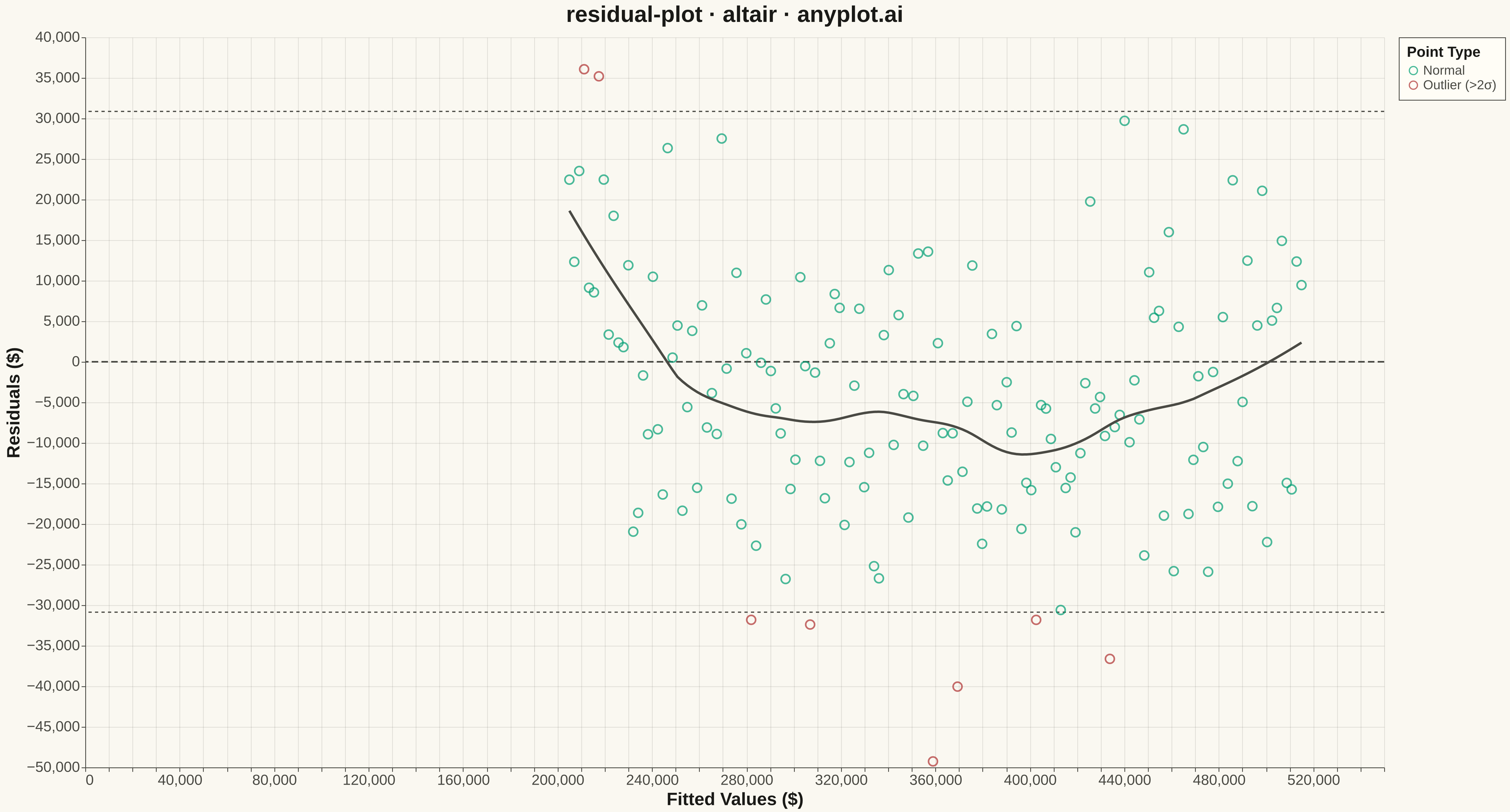
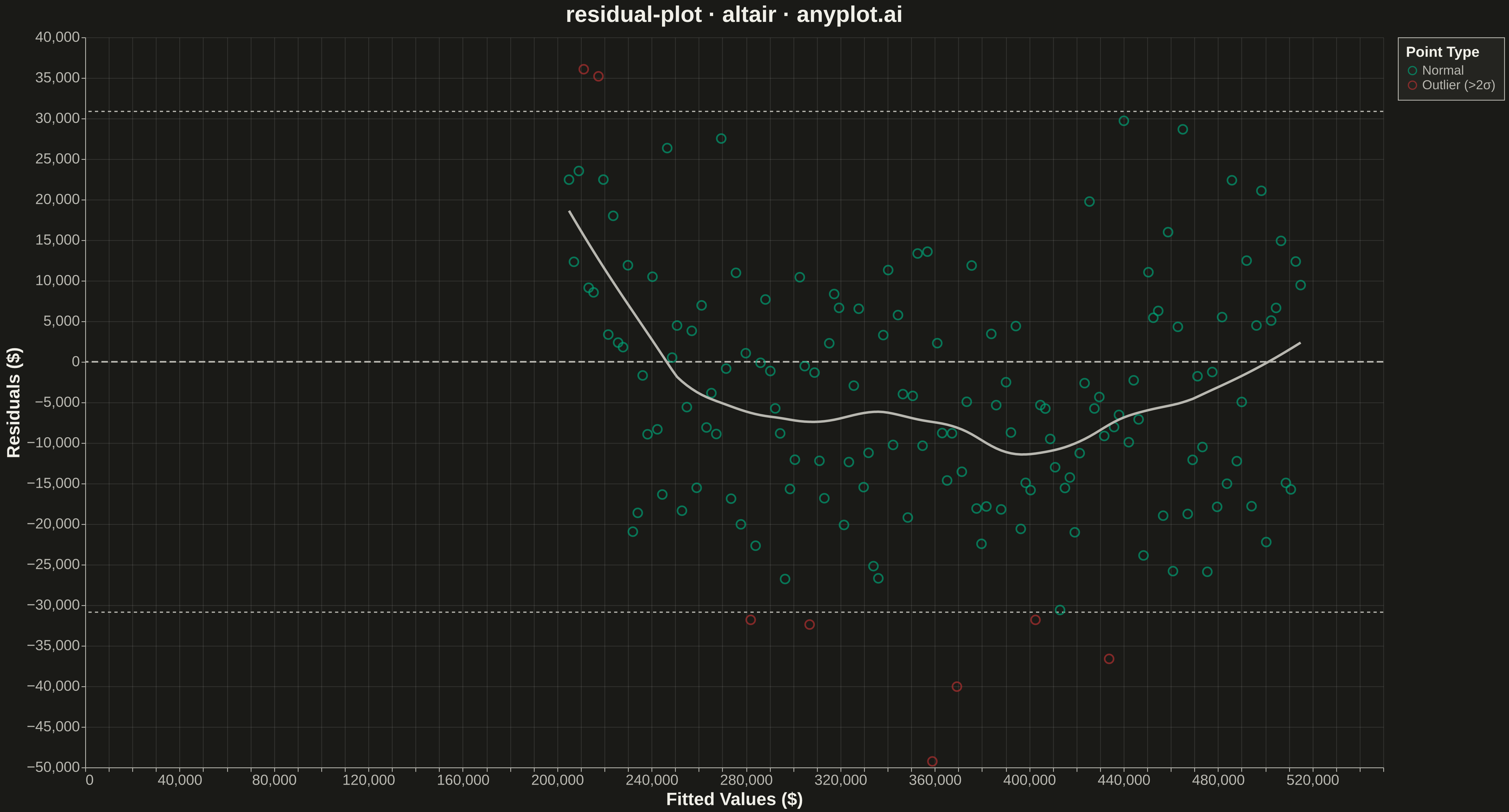
A residual plot displays the difference between observed and predicted values (residuals) against fitted values or an independent variable in regression analysis. This diagnostic visualization helps identify violations of regression assumptions including non-linearity, heteroscedasticity (non-constant variance), and outliers. A well-fitting model shows residuals randomly scattered around zero with no discernible pattern.
""" anyplot.ai
residual-plot: Residual Plot
Library: altair 6.1.0 | Python 3.13.13
Quality: 92/100 | Updated: 2026-05-10
"""

import os
import sys


# Remove script directory from path to avoid importing local altair.py
script_dir = os.path.dirname(os.path.abspath(__file__))
sys.path = [p for p in sys.path if os.path.abspath(p) != script_dir]

import altair as alt
import numpy as np
import pandas as pd


# Theme tokens
THEME = os.getenv("ANYPLOT_THEME", "light")
PAGE_BG = "#FAF8F1" if THEME == "light" else "#1A1A17"
ELEVATED_BG = "#FFFDF6" if THEME == "light" else "#242420"
INK = "#1A1A17" if THEME == "light" else "#F0EFE8"
INK_SOFT = "#4A4A44" if THEME == "light" else "#B8B7B0"

OKABE_ITO_1 = "#009E73"  # Brand green for main data
OUTLIER_COLOR = "#AE3030"  # imprint red — outliers (>2σ)

# Data: Simulate a linear regression scenario with some non-linearity
np.random.seed(42)
n = 150

# Generate realistic housing price prediction scenario
x = np.linspace(1000, 3000, n)  # House size in sq ft
noise = np.random.randn(n) * 15000
y_true = 50000 + 150 * x + 0.02 * (x - 2000) ** 2 + noise  # True prices with slight curvature
y_pred = 50000 + 155 * x  # Linear model predictions

residuals = y_true - y_pred
std_residual = np.std(residuals)

# Identify outliers (beyond ±2 standard deviations)
is_outlier = np.abs(residuals) > 2 * std_residual

# Create DataFrame
df = pd.DataFrame(
    {
        "Fitted Values ($)": y_pred,
        "Residuals ($)": residuals,
        "Outlier": np.where(is_outlier, "Outlier (>2σ)", "Normal"),
    }
)

# Base scatter plot with color encoding for outliers
scatter = (
    alt.Chart(df)
    .mark_point(size=120, opacity=0.7)
    .encode(
        x=alt.X("Fitted Values ($):Q", title="Fitted Values ($)", scale=alt.Scale(nice=True)),
        y=alt.Y("Residuals ($):Q", title="Residuals ($)", scale=alt.Scale(nice=True)),
        color=alt.Color(
            "Outlier:N",
            scale=alt.Scale(domain=["Normal", "Outlier (>2σ)"], range=[OKABE_ITO_1, OUTLIER_COLOR]),
            legend=alt.Legend(title="Point Type", titleFontSize=18, labelFontSize=16),
        ),
        tooltip=["Fitted Values ($):Q", "Residuals ($):Q", "Outlier:N"],
    )
)

# Zero reference line
zero_line = (
    alt.Chart(pd.DataFrame({"y": [0]})).mark_rule(color=INK_SOFT, strokeWidth=2, strokeDash=[8, 4]).encode(y="y:Q")
)

# ±2 standard deviation bands
bands_df = pd.DataFrame({"y": [2 * std_residual, -2 * std_residual], "label": ["+2σ", "-2σ"]})

band_lines = alt.Chart(bands_df).mark_rule(color=INK_SOFT, strokeWidth=1.5, strokeDash=[4, 4]).encode(y="y:Q")

# Add LOWESS-like trend using polynomial regression
loess_df = df.copy()
loess_df = loess_df.sort_values("Fitted Values ($)")

loess_line = (
    alt.Chart(loess_df)
    .transform_loess("Fitted Values ($)", "Residuals ($)", bandwidth=0.3)
    .mark_line(color=INK_SOFT, strokeWidth=3)
    .encode(x="Fitted Values ($):Q", y="Residuals ($):Q")
)

# Combine all layers
chart = (
    alt.layer(zero_line, band_lines, scatter, loess_line)
    .properties(
        width=1600,
        height=900,
        background=PAGE_BG,
        title=alt.Title(text="residual-plot · altair · anyplot.ai", fontSize=28, anchor="middle"),
    )
    .configure_view(strokeWidth=0, fill=PAGE_BG)
    .configure_axis(
        labelFontSize=18,
        titleFontSize=22,
        gridOpacity=0.10,
        domainColor=INK_SOFT,
        tickColor=INK_SOFT,
        gridColor=INK,
        labelColor=INK_SOFT,
        titleColor=INK,
    )
    .configure_title(color=INK)
    .configure_legend(
        fillColor=ELEVATED_BG, strokeColor=INK_SOFT, labelColor=INK_SOFT, titleColor=INK, orient="right", padding=10
    )
)

# Save outputs
chart.save(f"plot-{THEME}.png", scale_factor=3.0)
chart.save(f"plot-{THEME}.html")
Runnable source as JSON, for any HTTP client: https://api.anyplot.ai/specs/residual-plot/altair/code. Any spec id and library id listed in llms-full.txt fit the same URL shape; every URL below is complete and callable.
{
  "spec_id": "residual-plot",
  "language": "python",
  "library": "altair",
  "page": "https://anyplot.ai/residual-plot/python/altair",
  "hub": "https://anyplot.ai/residual-plot",
  "code_json": "https://api.anyplot.ai/specs/residual-plot/altair/code",
  "spec_json": "https://api.anyplot.ai/specs/residual-plot",
  "render_light_png": "https://storage.googleapis.com/anyplot-images/plots/residual-plot/python/altair/plot-light.png",
  "render_dark_png": "https://storage.googleapis.com/anyplot-images/plots/residual-plot/python/altair/plot-dark.png",
  "interactive_light_html": "https://storage.googleapis.com/anyplot-images/plots/residual-plot/python/altair/plot-light.html",
  "interactive_dark_html": "https://storage.googleapis.com/anyplot-images/plots/residual-plot/python/altair/plot-dark.html",
  "quality_score": 92.0,
  "license": "MIT",
  "guide": "https://anyplot.ai/llms.txt"
}
Part of Residual Plot on anyplot.ai.