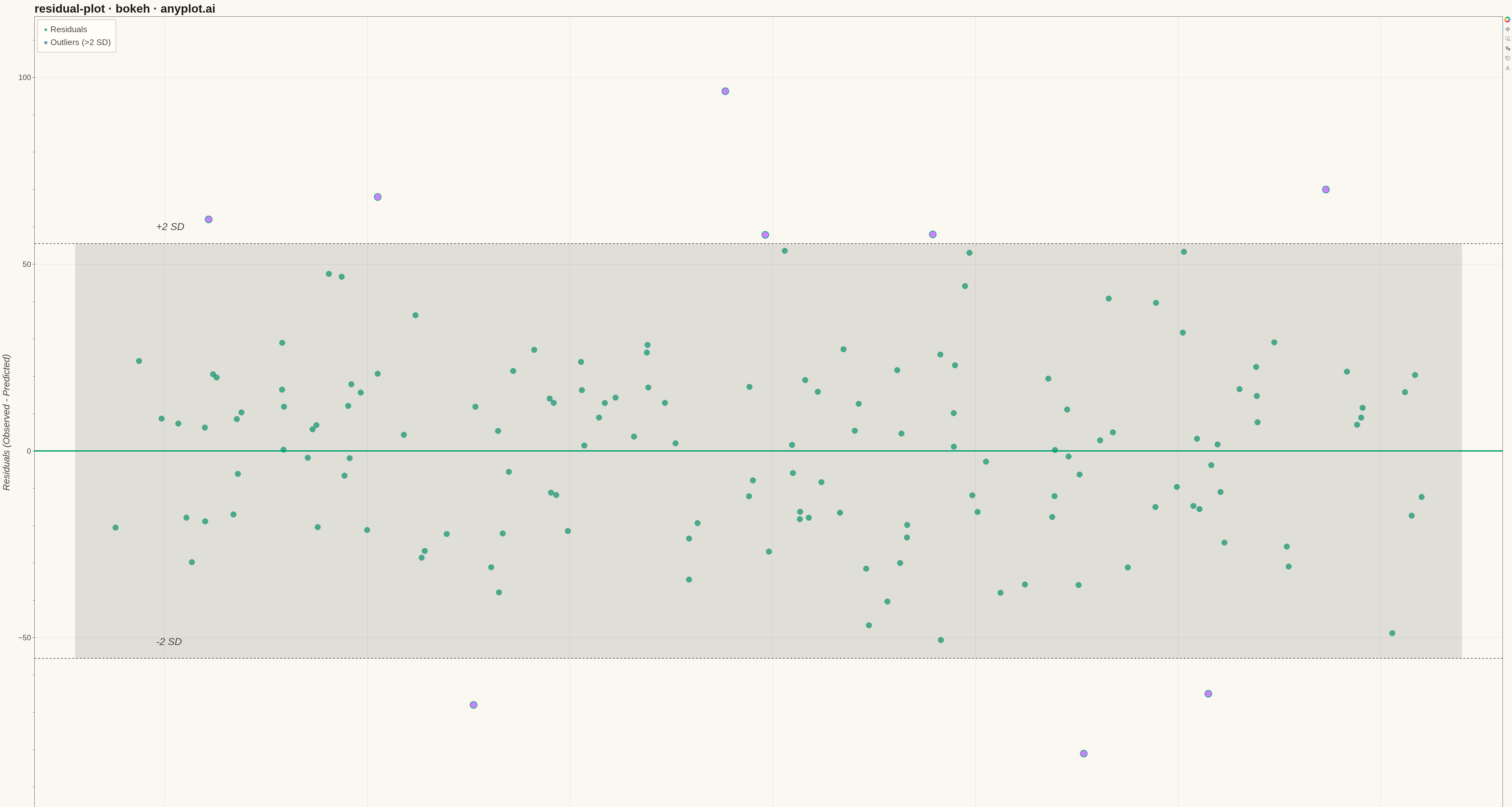
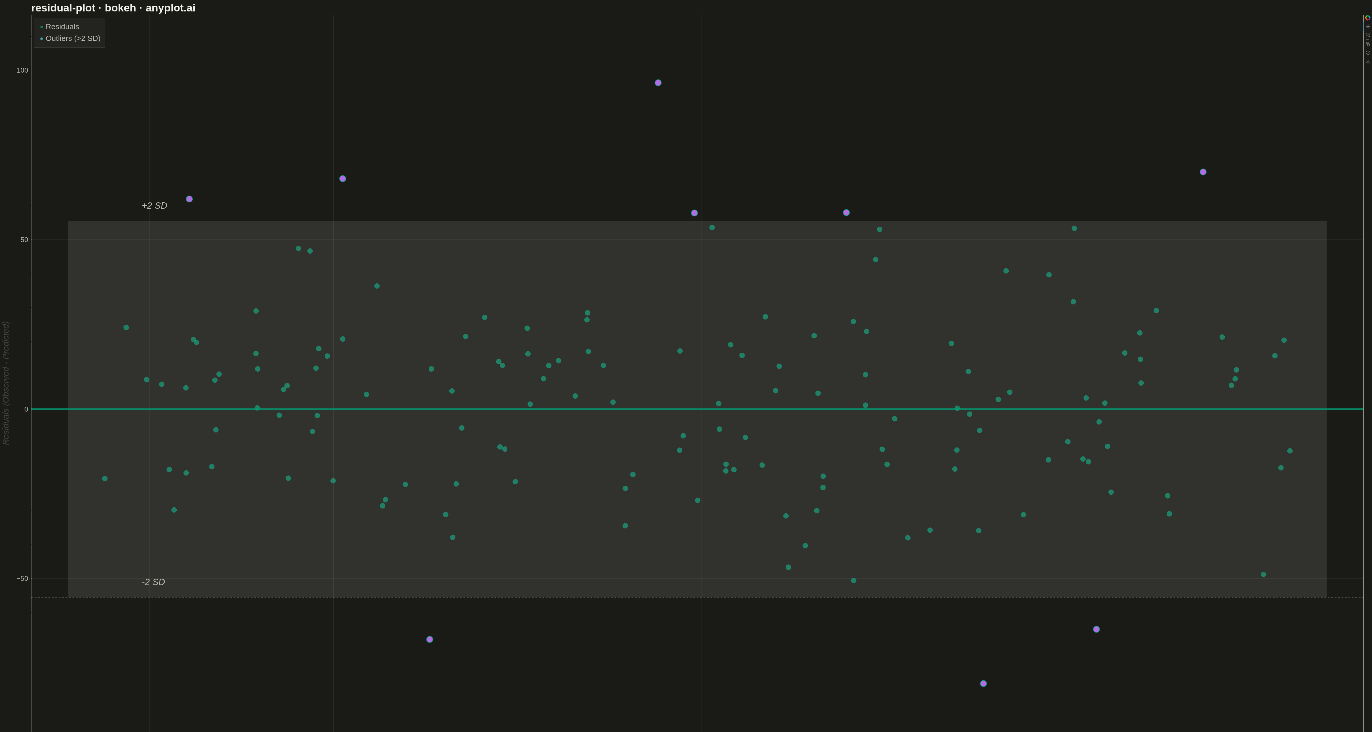
A residual plot displays the difference between observed and predicted values (residuals) against fitted values or an independent variable in regression analysis. This diagnostic visualization helps identify violations of regression assumptions including non-linearity, heteroscedasticity (non-constant variance), and outliers. A well-fitting model shows residuals randomly scattered around zero with no discernible pattern.
""" anyplot.ai
residual-plot: Residual Plot
Library: bokeh 3.9.0 | Python 3.13.13
Quality: 98/100 | Updated: 2026-05-10
"""

import os
import time
from pathlib import Path

import numpy as np
from bokeh.io import output_file, save
from bokeh.models import Band, ColumnDataSource, Label, Span
from bokeh.plotting import figure
from selenium import webdriver
from selenium.webdriver.chrome.options import Options


# Theme tokens
THEME = os.getenv("ANYPLOT_THEME", "light")
PAGE_BG = "#FAF8F1" if THEME == "light" else "#1A1A17"
ELEVATED_BG = "#FFFDF6" if THEME == "light" else "#242420"
INK = "#1A1A17" if THEME == "light" else "#F0EFE8"
INK_SOFT = "#4A4A44" if THEME == "light" else "#B8B7B0"

BRAND = "#009E73"  # Okabe-Ito position 1 (residuals)
OUTLIER_COLOR = "#C475FD"  # Okabe-Ito position 2 (outliers)

# Data - Linear regression example with realistic housing price prediction
np.random.seed(42)
n_points = 150

# Generate fitted values (predicted house prices in $1000s)
y_pred = np.linspace(150, 450, n_points) + np.random.randn(n_points) * 20

# Generate residuals with some heteroscedasticity pattern for demonstration
base_residuals = np.random.randn(n_points) * 25
# Add a few outliers beyond 2 standard deviations
outlier_indices = [10, 45, 89, 120, 140]
base_residuals[outlier_indices] = np.array([62, -68, 58, -65, 70])

residuals = base_residuals
y_true = y_pred + residuals

# Calculate statistics for reference bands
residual_std = np.std(residuals)
upper_band = 2 * residual_std
lower_band = -2 * residual_std

# Identify outliers (beyond ±2 standard deviations)
is_outlier = np.abs(residuals) > 2 * residual_std

# Prepare data sources
source_normal = ColumnDataSource(data={"x": y_pred[~is_outlier], "y": residuals[~is_outlier]})
source_outliers = ColumnDataSource(data={"x": y_pred[is_outlier], "y": residuals[is_outlier]})

# Band data for ±2 SD region
band_source = ColumnDataSource(
    data={
        "x": np.array([min(y_pred) - 10, max(y_pred) + 10]),
        "lower": np.array([lower_band, lower_band]),
        "upper": np.array([upper_band, upper_band]),
    }
)

# Create figure (4800x2700 for 16:9)
p = figure(
    width=4800,
    height=2700,
    title="residual-plot · bokeh · anyplot.ai",
    x_axis_label="Fitted Values (Predicted Price in $1000s)",
    y_axis_label="Residuals (Observed - Predicted)",
    tools="pan,wheel_zoom,box_zoom,reset,save",
    x_range=(min(y_pred) - 20, max(y_pred) + 20),
    y_range=(min(residuals) - 20, max(residuals) + 20),
)

# Add ±2 SD band (light fill with theme-adaptive color)
band = Band(
    base="x", lower="lower", upper="upper", source=band_source, fill_alpha=0.15, fill_color=INK_SOFT, line_width=0
)
p.add_layout(band)

# Add horizontal reference line at y=0
zero_line = Span(location=0, dimension="width", line_color=BRAND, line_width=4, line_dash="solid")
p.add_layout(zero_line)

# Add dashed lines at ±2 SD boundaries
upper_line = Span(location=upper_band, dimension="width", line_color=INK_SOFT, line_width=2, line_dash="dashed")
lower_line = Span(location=lower_band, dimension="width", line_color=INK_SOFT, line_width=2, line_dash="dashed")
p.add_layout(upper_line)
p.add_layout(lower_line)

# Plot normal points (Brand color)
p.scatter("x", "y", source=source_normal, size=18, color=BRAND, alpha=0.7, legend_label="Residuals")

# Plot outliers (Okabe-Ito color 2)
p.scatter(
    "x",
    "y",
    source=source_outliers,
    size=22,
    color=OUTLIER_COLOR,
    alpha=0.9,
    line_color=BRAND,
    line_width=2,
    legend_label="Outliers (>2 SD)",
)

# Add labels for ±2 SD bands (larger font for better visibility)
label_upper = Label(
    x=min(y_pred) + 10,
    y=upper_band + 3,
    text="+2 SD",
    text_font_size="24pt",
    text_color=INK_SOFT,
    text_font_style="italic",
)
label_lower = Label(
    x=min(y_pred) + 10,
    y=lower_band + 3,
    text="-2 SD",
    text_font_size="24pt",
    text_color=INK_SOFT,
    text_font_style="italic",
)
p.add_layout(label_upper)
p.add_layout(label_lower)

# Styling - Text sizes for 4800x2700 canvas
p.title.text_font_size = "28pt"
p.title.text_color = INK
p.xaxis.axis_label_text_font_size = "22pt"
p.yaxis.axis_label_text_font_size = "22pt"
p.xaxis.major_label_text_font_size = "18pt"
p.yaxis.major_label_text_font_size = "18pt"

# Grid styling
p.xgrid.grid_line_color = INK
p.ygrid.grid_line_color = INK
p.xgrid.grid_line_alpha = 0.10
p.ygrid.grid_line_alpha = 0.10

# Legend styling
p.legend.location = "top_left"
p.legend.label_text_font_size = "20pt"
p.legend.label_text_color = INK_SOFT
p.legend.background_fill_color = ELEVATED_BG
p.legend.border_line_color = INK_SOFT
p.legend.padding = 15
p.legend.spacing = 10

# Axis styling
p.xaxis.axis_line_color = INK_SOFT
p.yaxis.axis_line_color = INK_SOFT
p.xaxis.major_label_text_color = INK_SOFT
p.yaxis.major_label_text_color = INK_SOFT
p.xaxis.major_tick_line_color = INK_SOFT
p.yaxis.major_tick_line_color = INK_SOFT

# Background
p.background_fill_color = PAGE_BG
p.border_fill_color = PAGE_BG
p.outline_line_color = INK_SOFT

# Save HTML output
output_file(f"plot-{THEME}.html")
save(p)

# Screenshot with headless Chrome (Selenium)
W, H = 4800, 2700
opts = Options()
for arg in (
    "--headless=new",
    "--no-sandbox",
    "--disable-dev-shm-usage",
    "--disable-gpu",
    f"--window-size={W},{H}",
    "--hide-scrollbars",
):
    opts.add_argument(arg)
driver = webdriver.Chrome(options=opts)
driver.set_window_size(W, H)
driver.get(f"file://{Path(f'plot-{THEME}.html').resolve()}")
time.sleep(3)
driver.save_screenshot(f"plot-{THEME}.png")
driver.quit()
Runnable source as JSON, for any HTTP client: https://api.anyplot.ai/specs/residual-plot/bokeh/code. Any spec id and library id listed in llms-full.txt fit the same URL shape; every URL below is complete and callable.
{
  "spec_id": "residual-plot",
  "language": "python",
  "library": "bokeh",
  "page": "https://anyplot.ai/residual-plot/python/bokeh",
  "hub": "https://anyplot.ai/residual-plot",
  "code_json": "https://api.anyplot.ai/specs/residual-plot/bokeh/code",
  "spec_json": "https://api.anyplot.ai/specs/residual-plot",
  "render_light_png": "https://storage.googleapis.com/anyplot-images/plots/residual-plot/python/bokeh/plot-light.png",
  "render_dark_png": "https://storage.googleapis.com/anyplot-images/plots/residual-plot/python/bokeh/plot-dark.png",
  "interactive_light_html": "https://storage.googleapis.com/anyplot-images/plots/residual-plot/python/bokeh/plot-light.html",
  "interactive_dark_html": "https://storage.googleapis.com/anyplot-images/plots/residual-plot/python/bokeh/plot-dark.html",
  "quality_score": 98.0,
  "license": "MIT",
  "guide": "https://anyplot.ai/llms.txt"
}
Part of Residual Plot on anyplot.ai.