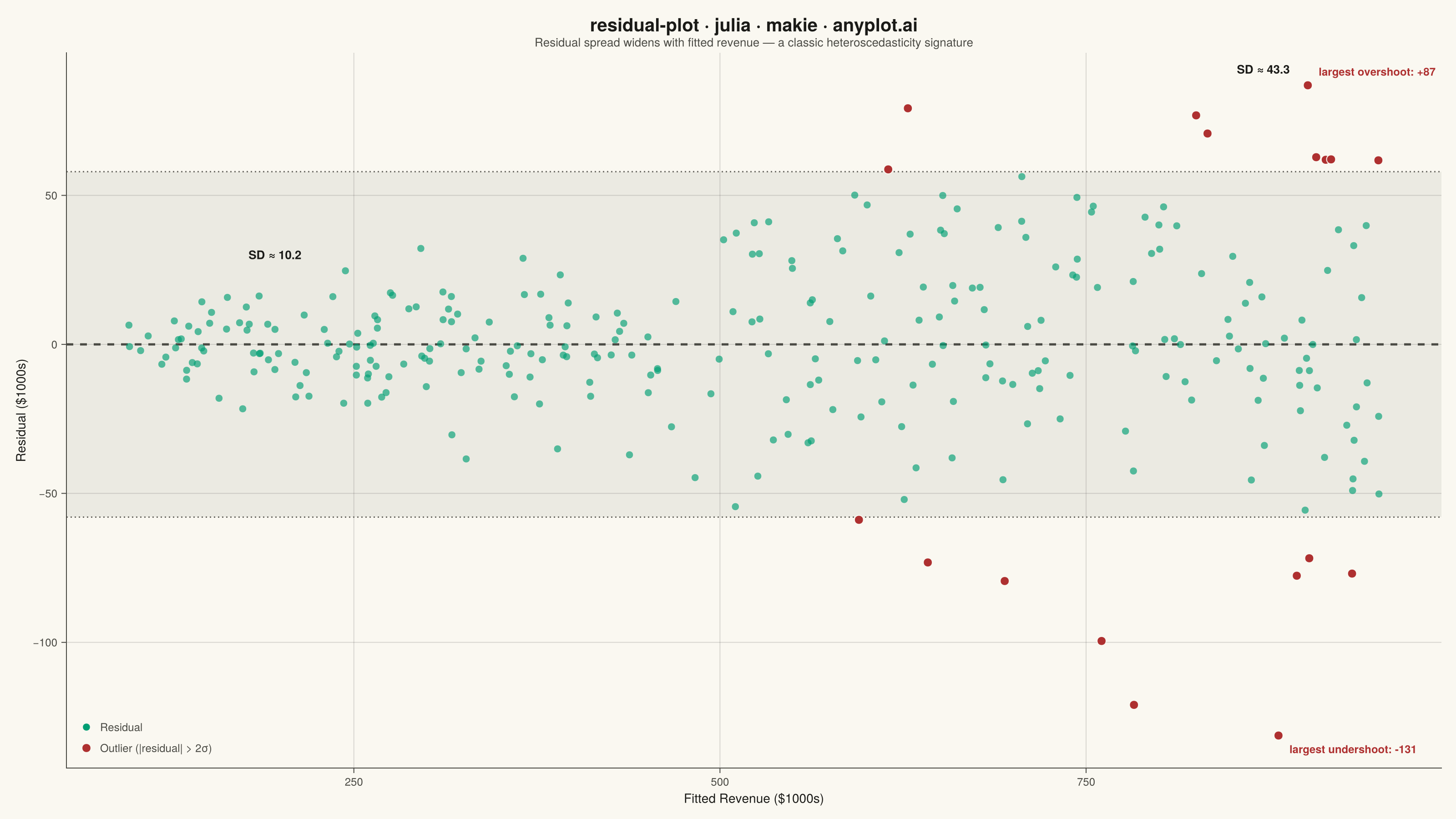
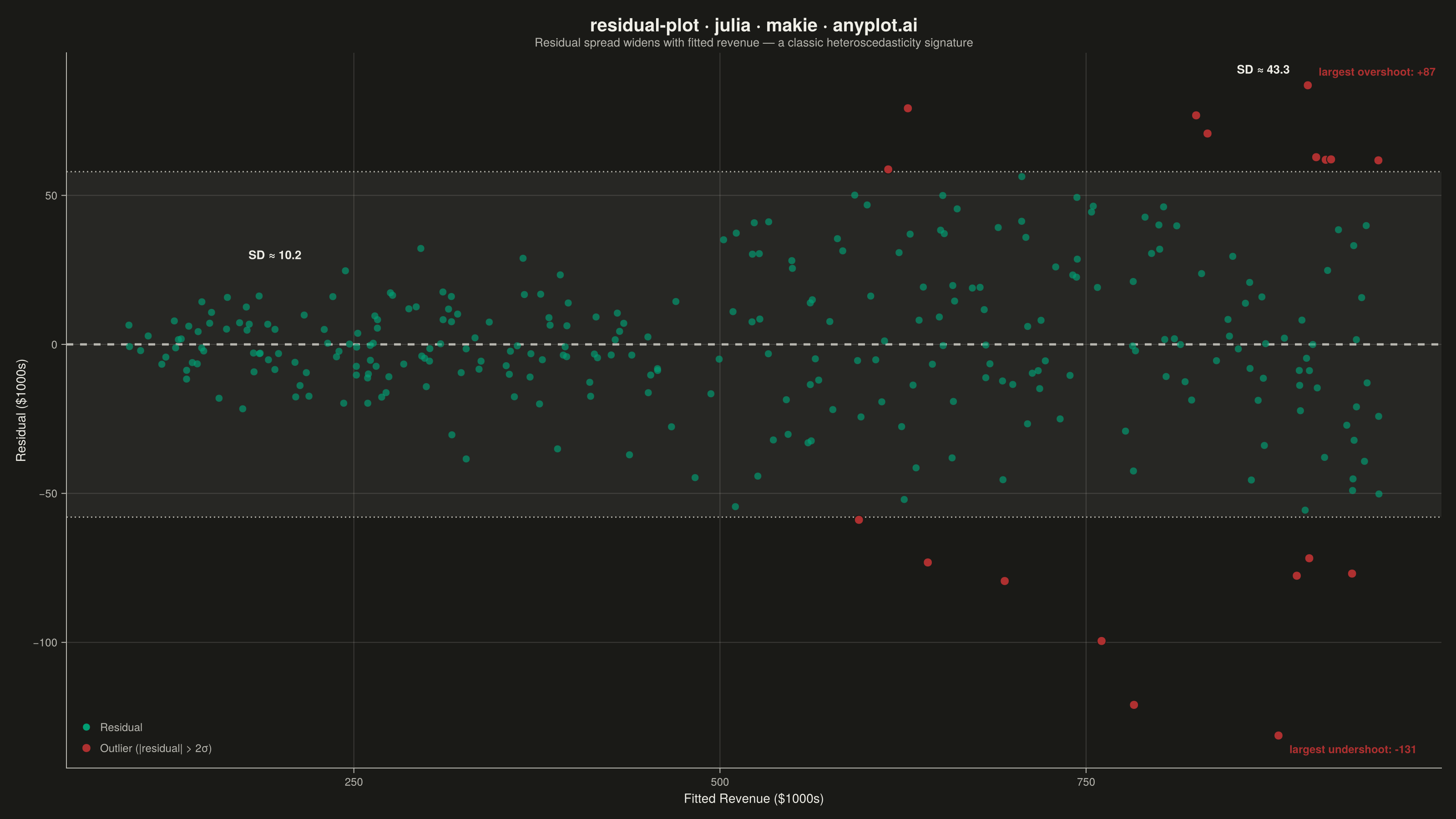
The same plot in 14 other libraries — Python: Altair, Bokeh, lets-plot, Matplotlib, Plotly, plotnine, Pygal, Seaborn; R: ggplot2; JavaScript: Chart.js, D3.js, Apache ECharts, Highcharts, MUI X Charts. Compare all 15 side by side: Residual Plot in Python, R, Julia and JavaScript.
A residual plot displays the difference between observed and predicted values (residuals) against fitted values in regression analysis. This diagnostic visualization helps identify violations of regression assumptions including non-linearity, heteroscedasticity (non-constant variance), and outliers. A well-fitting model shows residuals randomly scattered around zero with no discernible pattern.
# anyplot.ai
# residual-plot: Residual Plot
# Library: makie 0.21.9 | Julia 1.11.9
# Quality: 94/100 | Created: 2026-09-05

using CairoMakie
using Colors
using Random
using Statistics

Random.seed!(42)

# --- Theme tokens -----------------------------------------------------------
const THEME    = get(ENV, "ANYPLOT_THEME", "light")
const PAGE_BG  = THEME == "light" ? colorant"#FAF8F1" : colorant"#1A1A17"
const INK      = THEME == "light" ? colorant"#1A1A17" : colorant"#F0EFE8"
const INK_SOFT = THEME == "light" ? colorant"#4A4A44" : colorant"#B8B7B0"
const MUTED    = THEME == "light" ? colorant"#6B6A63" : colorant"#A8A79F"
const IMPRINT_PALETTE = [
    colorant"#009E73", colorant"#C475FD", colorant"#4467A3", colorant"#BD8233",
    colorant"#AE3030", colorant"#2ABCCD", colorant"#954477", colorant"#99B314",
]

# --- Data ---------------------------------------------------------------
# Advertising spend ($1000s) predicting weekly revenue ($1000s). The true
# relationship is linear but noise variance grows with spend, so a simple
# OLS fit leaves heteroscedastic residuals — exactly what this plot is
# meant to expose.
n = 300
ad_spend = sort(rand(n) .* 190 .+ 10)
noise_scale = 1.0 .+ 0.06 .* ad_spend
revenue = 50 .+ 4.5 .* ad_spend .+ randn(n) .* noise_scale .* 3.5

spend_mean = mean(ad_spend)
revenue_mean = mean(revenue)
slope = sum((ad_spend .- spend_mean) .* (revenue .- revenue_mean)) / sum((ad_spend .- spend_mean) .^ 2)
intercept = revenue_mean - slope * spend_mean
fitted_revenue = intercept .+ slope .* ad_spend
residuals = revenue .- fitted_revenue

resid_std = std(residuals)
is_outlier = abs.(residuals) .> 2 * resid_std

# Quantify the heteroscedasticity story: local spread in the narrow (low
# fitted-revenue) and wide (high fitted-revenue) quartiles, called out
# directly on the plot instead of leaving the funnel shape to speak for itself.
lo_cut = quantile(fitted_revenue, 0.25)
hi_cut = quantile(fitted_revenue, 0.75)
lo_mask = fitted_revenue .< lo_cut
hi_mask = fitted_revenue .> hi_cut
lo_sigma = std(residuals[lo_mask])
hi_sigma = std(residuals[hi_mask])
lo_anchor_x = quantile(fitted_revenue[lo_mask], 0.5)
hi_anchor_x = quantile(fitted_revenue[hi_mask], 0.5)
lo_anchor_y = maximum(residuals[lo_mask])
hi_anchor_y = maximum(residuals[hi_mask])

idx_max = argmax(residuals)
idx_min = argmin(residuals)

# --- Plot -----------------------------------------------------------------
fig = Figure(
    resolution      = (1600, 900),
    fontsize        = 14,
    backgroundcolor = PAGE_BG,
)

ax = Axis(
    fig[1, 1];
    title              = "residual-plot · julia · makie · anyplot.ai",
    titlesize          = 20,
    titlecolor         = INK,
    subtitle           = "Residual spread widens with fitted revenue — a classic heteroscedasticity signature",
    subtitlesize       = 13,
    subtitlecolor      = INK_SOFT,
    xlabel             = "Fitted Revenue (\$1000s)",
    ylabel             = "Residual (\$1000s)",
    xlabelsize         = 14,
    ylabelsize         = 14,
    xlabelcolor        = INK,
    ylabelcolor        = INK,
    xticklabelsize     = 12,
    yticklabelsize     = 12,
    xticklabelcolor    = INK_SOFT,
    yticklabelcolor    = INK_SOFT,
    xtickcolor         = INK_SOFT,
    ytickcolor         = INK_SOFT,
    backgroundcolor    = PAGE_BG,
    topspinevisible    = false,
    rightspinevisible  = false,
    leftspinecolor     = INK_SOFT,
    bottomspinecolor   = INK_SOFT,
    xgridcolor         = RGBAf(INK.r, INK.g, INK.b, 0.15),
    ygridcolor         = RGBAf(INK.r, INK.g, INK.b, 0.15),
    xminorgridvisible  = false,
    yminorgridvisible  = false,
)

hspan!(ax, -2 * resid_std, 2 * resid_std; color = RGBAf(MUTED.r, MUTED.g, MUTED.b, 0.10))
hlines!(ax, [-2resid_std, 2resid_std]; color = MUTED, linewidth = 1.5, linestyle = :dot)
hlines!(ax, [0]; color = INK_SOFT, linewidth = 2.5, linestyle = :dash)

scatter!(
    ax, fitted_revenue[.!is_outlier], residuals[.!is_outlier];
    color = IMPRINT_PALETTE[1], markersize = 11, alpha = 0.65, strokewidth = 0,
    label = "Residual",
)
scatter!(
    ax, fitted_revenue[is_outlier], residuals[is_outlier];
    color = IMPRINT_PALETTE[5], markersize = 14, strokewidth = 1, strokecolor = PAGE_BG,
    label = "Outlier (|residual| > 2σ)",
)

# Quantified spread callouts anchored directly in data coordinates — makes the
# heteroscedasticity insight explicit rather than leaving the funnel to speak
# for itself.
text!(
    ax, lo_anchor_x, lo_anchor_y;
    text = "SD ≈ $(round(lo_sigma, digits = 1))", color = INK, fontsize = 13,
    font = :bold, align = (:center, :bottom), offset = (0, 10),
)
text!(
    ax, hi_anchor_x, hi_anchor_y;
    text = "SD ≈ $(round(hi_sigma, digits = 1))", color = INK, fontsize = 13,
    font = :bold, align = (:center, :bottom), offset = (0, 10),
)

# Label the two most extreme outliers to give the outlier cluster a
# deliberate focal point instead of leaving it as undifferentiated dots.
text!(
    ax, fitted_revenue[idx_max], residuals[idx_max];
    text = "largest overshoot: +$(round(Int, residuals[idx_max]))",
    color = IMPRINT_PALETTE[5], fontsize = 12, font = :bold,
    align = (:left, :bottom), offset = (12, 8),
)
text!(
    ax, fitted_revenue[idx_min], residuals[idx_min];
    text = "largest undershoot: $(round(Int, residuals[idx_min]))",
    color = IMPRINT_PALETTE[5], fontsize = 12, font = :bold,
    align = (:left, :top), offset = (12, -8),
)

axislegend(
    ax;
    position = :lb,
    labelcolor = INK_SOFT,
    labelsize = 12,
    framevisible = false,
    backgroundcolor = :transparent,
)

# --- Save -------------------------------------------------------------------
save("plot-$(THEME).png", fig; px_per_unit = 2)
Runnable source as JSON, for any HTTP client: https://api.anyplot.ai/specs/residual-plot/makie/code. Any spec id and library id listed in llms-full.txt fit the same URL shape; every URL below is complete and callable.
{
  "spec_id": "residual-plot",
  "language": "julia",
  "library": "makie",
  "page": "https://anyplot.ai/residual-plot/julia/makie",
  "hub": "https://anyplot.ai/residual-plot",
  "code_json": "https://api.anyplot.ai/specs/residual-plot/makie/code",
  "spec_json": "https://api.anyplot.ai/specs/residual-plot",
  "render_light_png": "https://storage.googleapis.com/anyplot-images/plots/residual-plot/julia/makie/plot-light.png",
  "render_dark_png": "https://storage.googleapis.com/anyplot-images/plots/residual-plot/julia/makie/plot-dark.png",
  "quality_score": 94.0,
  "license": "MIT",
  "guide": "https://anyplot.ai/llms.txt"
}
Part of Residual Plot on anyplot.ai.