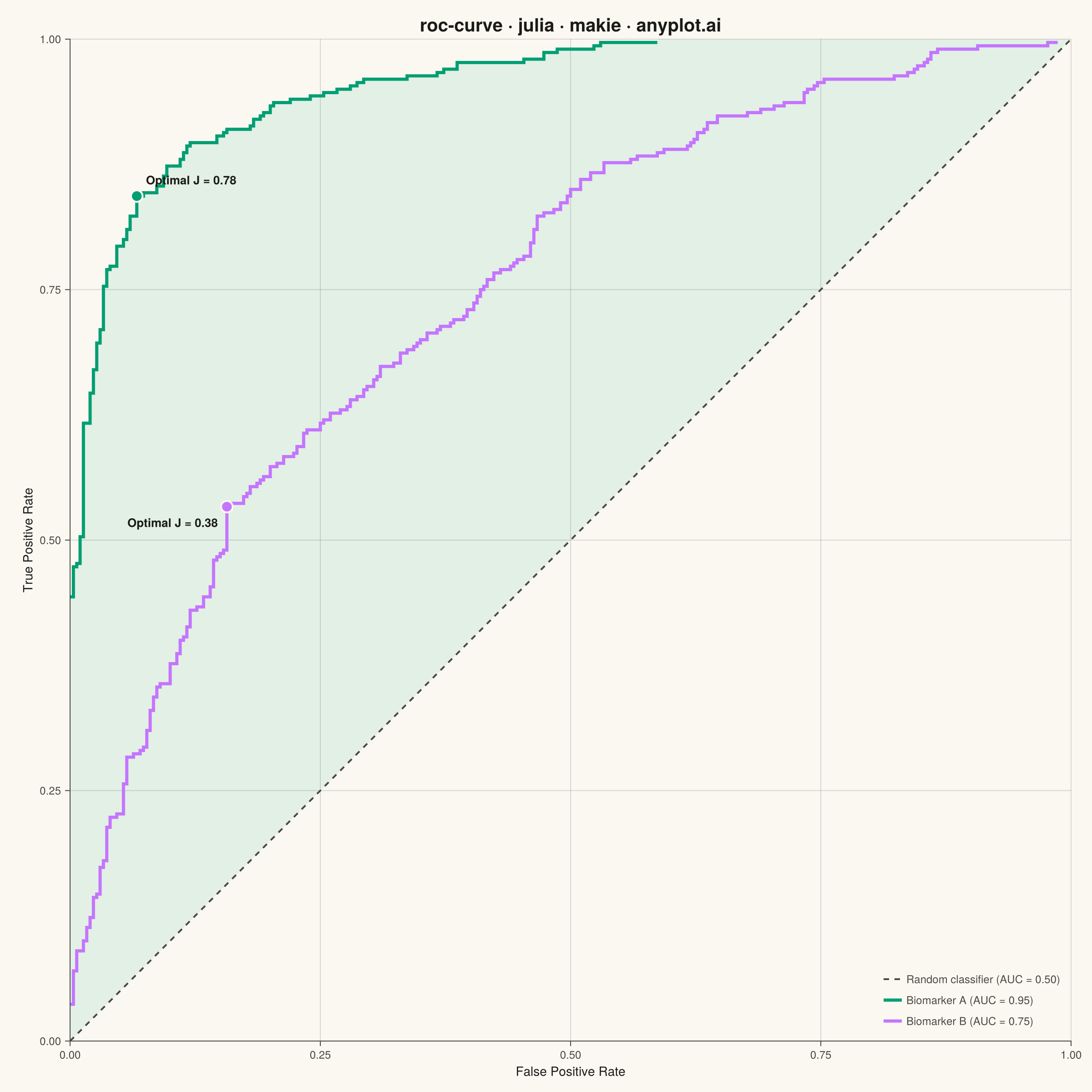
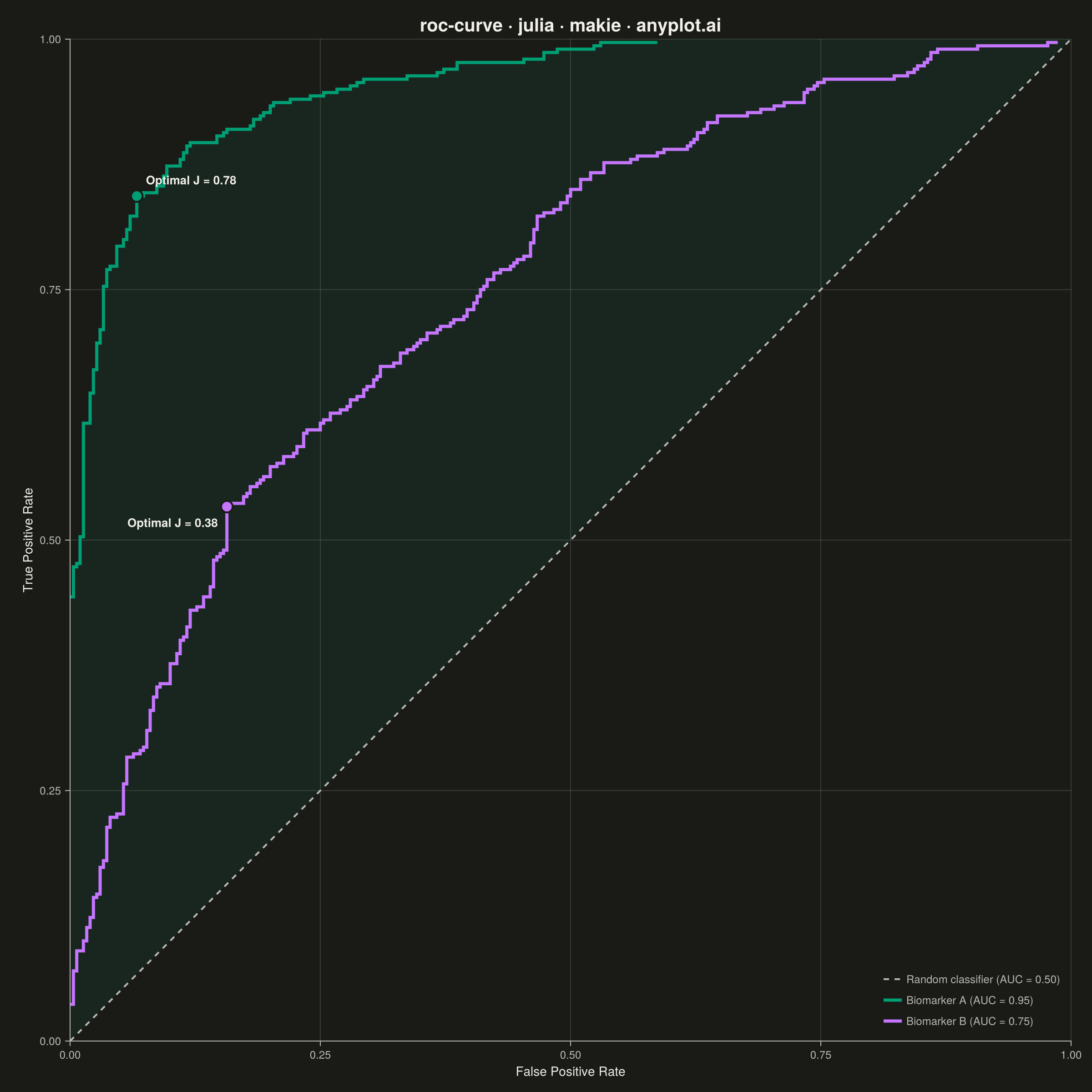
The same plot in 14 other libraries — Python: Altair, Bokeh, lets-plot, Matplotlib, Plotly, plotnine, Pygal, Seaborn; R: ggplot2; JavaScript: Chart.js, D3.js, Apache ECharts, Highcharts, MUI X Charts. Compare all 15 side by side: ROC Curve with AUC in Python, R, Julia and JavaScript.
A Receiver Operating Characteristic (ROC) curve visualizes the performance of a binary classifier by plotting the True Positive Rate (TPR) against the False Positive Rate (FPR) at various classification thresholds. The Area Under the Curve (AUC) provides a single metric summarizing model performance, where 1.0 indicates perfect classification and 0.5 represents random guessing.
# anyplot.ai
# roc-curve: ROC Curve with AUC
# Library: makie 0.21.9 | Julia 1.11.9
# Quality: 88/100 | Created: 2026-09-05

using CairoMakie
using Colors
using Random

Random.seed!(42)

# --- Theme tokens ------------------------------------------------------------
THEME    = get(ENV, "ANYPLOT_THEME", "light")
PAGE_BG  = THEME == "light" ? colorant"#FAF8F1" : colorant"#1A1A17"
INK      = THEME == "light" ? colorant"#1A1A17" : colorant"#F0EFE8"
INK_SOFT = THEME == "light" ? colorant"#4A4A44" : colorant"#B8B7B0"
IMPRINT_PALETTE = [
    colorant"#009E73",  # 1 — brand green, always first series
    colorant"#C475FD",  # 2 — lavender
]

# --- Data: two diagnostic biomarkers vs. disease status ----------------------
n_healthy = 300
n_disease = 300

scores_healthy_a = randn(n_healthy) .* 1.0 .+ 0.0
scores_disease_a = randn(n_disease) .* 1.0 .+ 2.2

scores_healthy_b = randn(n_healthy) .* 1.2 .+ 0.0
scores_disease_b = randn(n_disease) .* 1.2 .+ 1.2

# ROC curve for biomarker A: sweep the combined score axis from high to low,
# accumulating hits (disease) and misses (healthy) as the threshold falls.
labels_a = vcat(ones(Int, n_disease), zeros(Int, n_healthy))
scores_a = vcat(scores_disease_a, scores_healthy_a)
order_a = sortperm(scores_a; rev = true)
sorted_labels_a = labels_a[order_a]
tpr_a = vcat(0.0, cumsum(sorted_labels_a) ./ n_disease)
fpr_a = vcat(0.0, cumsum(1 .- sorted_labels_a) ./ n_healthy)
auc_a = sum(diff(fpr_a) .* (tpr_a[2:end] .+ tpr_a[1:(end - 1)]) ./ 2)

# ROC curve for biomarker B
labels_b = vcat(ones(Int, n_disease), zeros(Int, n_healthy))
scores_b = vcat(scores_disease_b, scores_healthy_b)
order_b = sortperm(scores_b; rev = true)
sorted_labels_b = labels_b[order_b]
tpr_b = vcat(0.0, cumsum(sorted_labels_b) ./ n_disease)
fpr_b = vcat(0.0, cumsum(1 .- sorted_labels_b) ./ n_healthy)
auc_b = sum(diff(fpr_b) .* (tpr_b[2:end] .+ tpr_b[1:(end - 1)]) ./ 2)

# Optimal operating point per curve (Youden's J statistic: max(TPR - FPR))
j_a = tpr_a .- fpr_a
opt_idx_a = argmax(j_a)
opt_fpr_a, opt_tpr_a = fpr_a[opt_idx_a], tpr_a[opt_idx_a]

j_b = tpr_b .- fpr_b
opt_idx_b = argmax(j_b)
opt_fpr_b, opt_tpr_b = fpr_b[opt_idx_b], tpr_b[opt_idx_b]

# --- Plot ----------------------------------------------------------------
fig = Figure(
    size = (1200, 1200),
    fontsize = 14,
    backgroundcolor = PAGE_BG,
)

ax = Axis(
    fig[1, 1];
    title = "roc-curve · julia · makie · anyplot.ai",
    titlesize = 20,
    titlecolor = INK,
    xlabel = "False Positive Rate",
    ylabel = "True Positive Rate",
    xlabelsize = 14,
    ylabelsize = 14,
    xlabelcolor = INK,
    ylabelcolor = INK,
    xticklabelsize = 12,
    yticklabelsize = 12,
    xticklabelcolor = INK_SOFT,
    yticklabelcolor = INK_SOFT,
    xtickcolor = INK_SOFT,
    ytickcolor = INK_SOFT,
    backgroundcolor = PAGE_BG,
    aspect = 1,
    limits = (0, 1, 0, 1),
    xticks = 0:0.25:1,
    yticks = 0:0.25:1,
    topspinevisible = false,
    rightspinevisible = false,
    leftspinecolor = INK_SOFT,
    bottomspinecolor = INK_SOFT,
    xgridcolor = RGBAf(INK.r, INK.g, INK.b, 0.15),
    ygridcolor = RGBAf(INK.r, INK.g, INK.b, 0.15),
    xminorgridvisible = false,
    yminorgridvisible = false,
)

# Shade the area between the better-performing curve (Biomarker A) and the
# diagonal to visualize its AUC advantage over random guessing
band!(ax, fpr_a, fpr_a, tpr_a; color = (IMPRINT_PALETTE[1], 0.09))

lines!(
    ax, [0.0, 1.0], [0.0, 1.0];
    color = INK_SOFT, linestyle = :dash, linewidth = 2.0,
    label = "Random classifier (AUC = 0.50)",
)
lines!(
    ax, fpr_a, tpr_a;
    color = IMPRINT_PALETTE[1], linewidth = 3.5,
    label = "Biomarker A (AUC = $(round(auc_a; digits = 2)))",
)
lines!(
    ax, fpr_b, tpr_b;
    color = IMPRINT_PALETTE[2], linewidth = 3.5,
    label = "Biomarker B (AUC = $(round(auc_b; digits = 2)))",
)

# Mark each curve's optimal operating point (Youden's J statistic)
scatter!(
    ax, [opt_fpr_a], [opt_tpr_a];
    color = IMPRINT_PALETTE[1], markersize = 18, strokewidth = 2.0, strokecolor = PAGE_BG,
)
text!(
    ax, opt_fpr_a, opt_tpr_a;
    text = "Optimal J = $(round(j_a[opt_idx_a]; digits = 2))",
    color = INK, fontsize = 13, font = :bold, align = (:left, :bottom), offset = (10, 10),
)
scatter!(
    ax, [opt_fpr_b], [opt_tpr_b];
    color = IMPRINT_PALETTE[2], markersize = 18, strokewidth = 2.0, strokecolor = PAGE_BG,
)
text!(
    ax, opt_fpr_b, opt_tpr_b;
    text = "Optimal J = $(round(j_b[opt_idx_b]; digits = 2))",
    color = INK, fontsize = 13, font = :bold, align = (:right, :top), offset = (-10, -10),
)

axislegend(ax; position = :rb, labelsize = 12, labelcolor = INK_SOFT, framevisible = false)

# --- Save ----------------------------------------------------------------
save("plot-$(THEME).png", fig; px_per_unit = 2)
Runnable source as JSON, for any HTTP client: https://api.anyplot.ai/specs/roc-curve/makie/code. Any spec id and library id listed in llms-full.txt fit the same URL shape; every URL below is complete and callable.
{
  "spec_id": "roc-curve",
  "language": "julia",
  "library": "makie",
  "page": "https://anyplot.ai/roc-curve/julia/makie",
  "hub": "https://anyplot.ai/roc-curve",
  "code_json": "https://api.anyplot.ai/specs/roc-curve/makie/code",
  "spec_json": "https://api.anyplot.ai/specs/roc-curve",
  "render_light_png": "https://storage.googleapis.com/anyplot-images/plots/roc-curve/julia/makie/plot-light.png",
  "render_dark_png": "https://storage.googleapis.com/anyplot-images/plots/roc-curve/julia/makie/plot-dark.png",
  "quality_score": 88.0,
  "license": "MIT",
  "guide": "https://anyplot.ai/llms.txt"
}
Part of ROC Curve with AUC on anyplot.ai.