The same plot in 14 other libraries — Python: Altair, Bokeh, lets-plot, Matplotlib, Plotly, plotnine, Pygal, Seaborn; Julia: Makie.jl; JavaScript: Chart.js, D3.js, Apache ECharts, Highcharts, MUI X Charts. Compare all 15 side by side: ROC Curve with AUC in Python, R, Julia and JavaScript.
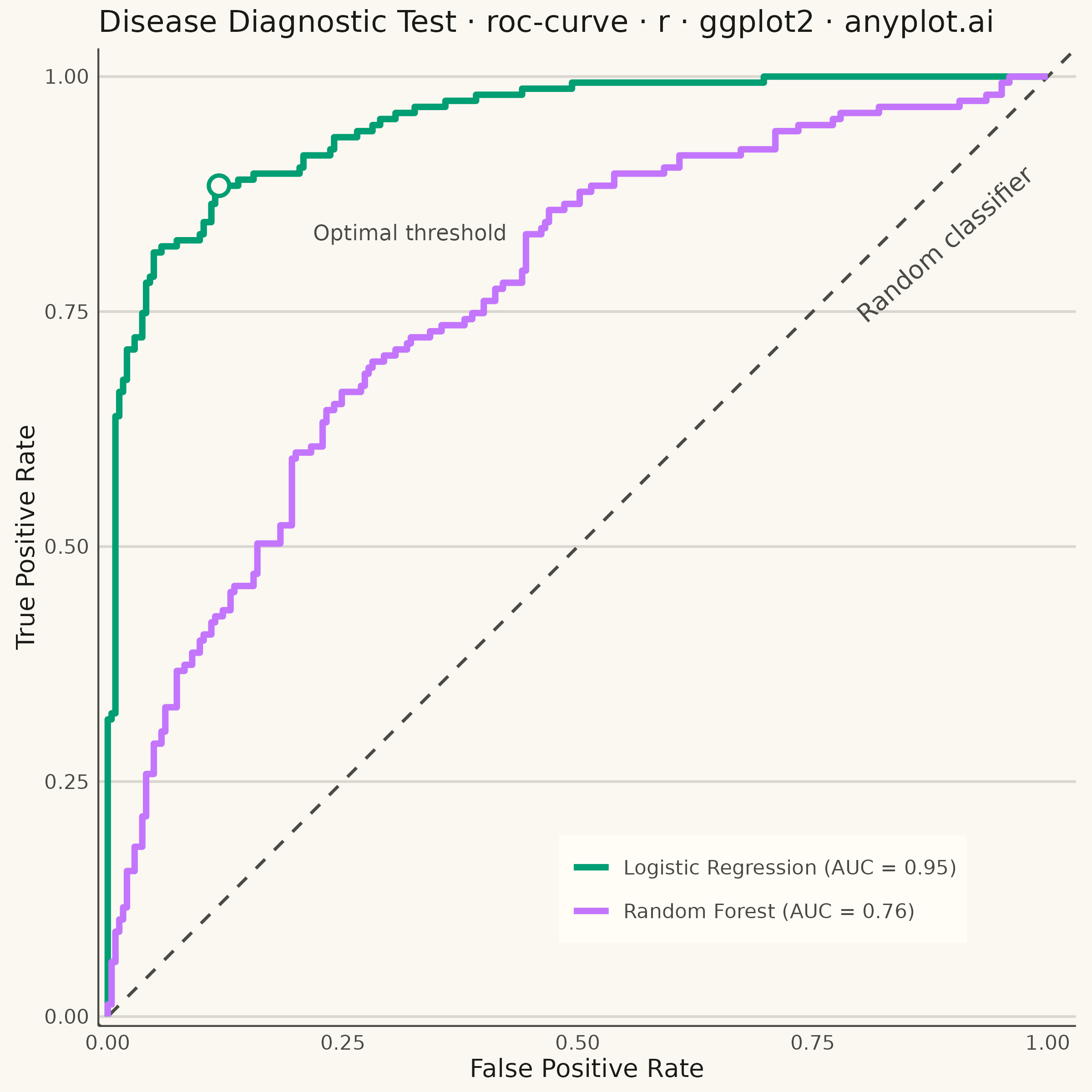
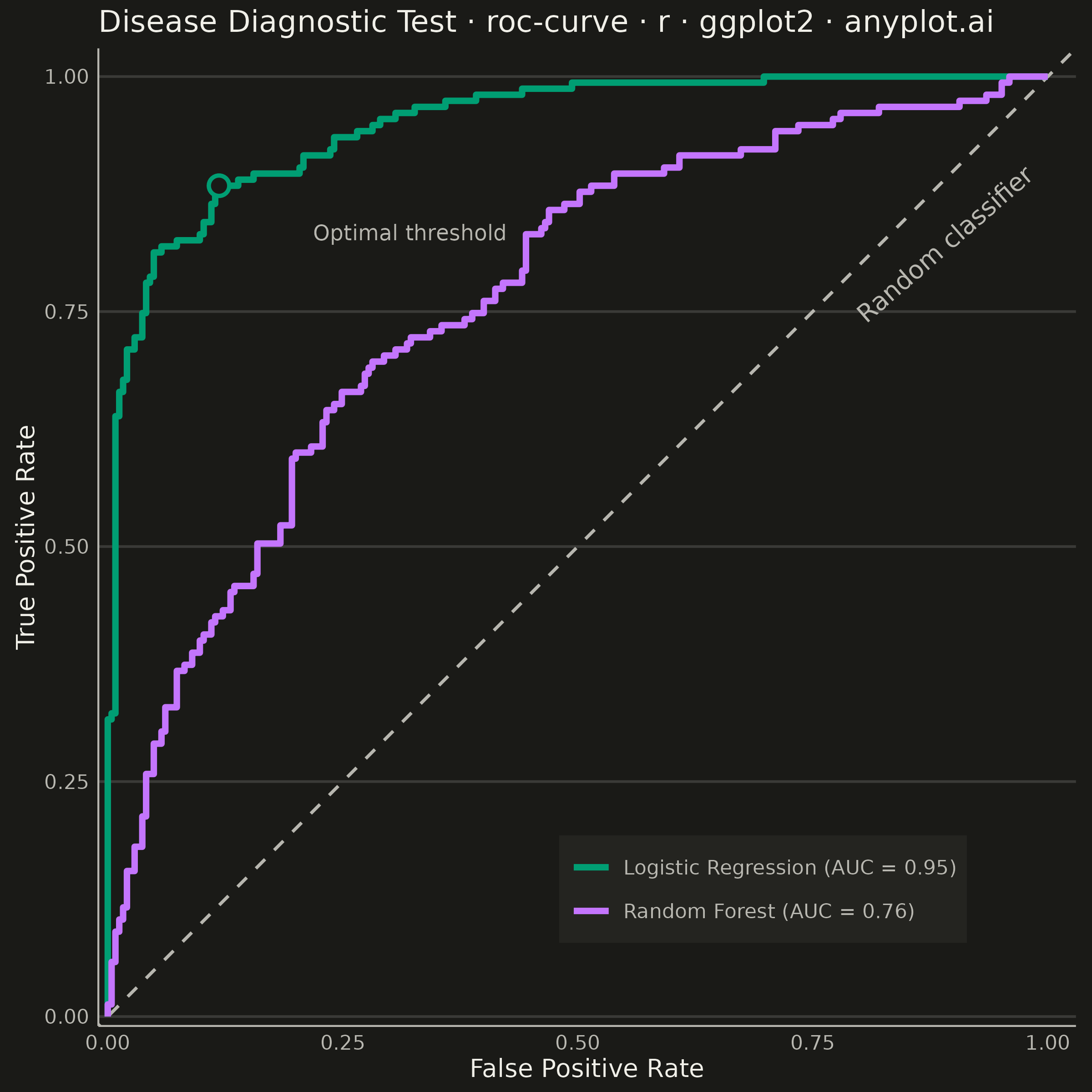
A Receiver Operating Characteristic (ROC) curve visualizes the performance of a binary classifier by plotting the True Positive Rate (TPR) against the False Positive Rate (FPR) at various classification thresholds. The Area Under the Curve (AUC) provides a single metric summarizing model performance, where 1.0 indicates perfect classification and 0.5 represents random guessing.
#' anyplot.ai
#' roc-curve: ROC Curve with AUC
#' Library: ggplot2 3.5.1 | R 4.4.1
#' Quality: 91/100 | Created: 2026-09-05

library(ggplot2)
library(dplyr)
library(ragg)
library(scales)

set.seed(42)

# --- Theme tokens -------------------------------------------------------
THEME       <- Sys.getenv("ANYPLOT_THEME", "light")
PAGE_BG     <- if (THEME == "light") "#FAF8F1" else "#1A1A17"
ELEVATED_BG <- if (THEME == "light") "#FFFDF6" else "#242420"
INK         <- if (THEME == "light") "#1A1A17" else "#F0EFE8"
INK_SOFT    <- if (THEME == "light") "#4A4A44" else "#B8B7B0"
IMPRINT_PALETTE <- c("#009E73", "#C475FD", "#4467A3", "#BD8233",
                     "#AE3030", "#2ABCCD", "#954477", "#99B314")

# --- Data -----------------------------------------------------------------
# Diagnostic test scores for two candidate classifiers separating
# disease-positive from disease-negative patients.
n_patients <- 400
disease <- rbinom(n_patients, 1, 0.4)

score_logistic <- ifelse(disease == 1,
                          rnorm(n_patients, mean = 2.2, sd = 1.0),
                          rnorm(n_patients, mean = 0.0, sd = 1.0))
score_forest <- ifelse(disease == 1,
                        rnorm(n_patients, mean = 1.2, sd = 1.1),
                        rnorm(n_patients, mean = 0.0, sd = 1.1))

roc_points <- function(scores, labels) {
  thresholds <- sort(unique(c(scores, Inf, -Inf)), decreasing = TRUE)
  n_pos <- sum(labels == 1)
  n_neg <- sum(labels == 0)
  tpr <- sapply(thresholds, function(t) sum(scores >= t & labels == 1) / n_pos)
  fpr <- sapply(thresholds, function(t) sum(scores >= t & labels == 0) / n_neg)
  tibble::tibble(fpr = fpr, tpr = tpr)
}

model_names <- c("Logistic Regression", "Random Forest")

roc_df <- bind_rows(
  roc_points(score_logistic, disease) %>% mutate(model = model_names[1]),
  roc_points(score_forest, disease) %>% mutate(model = model_names[2])
) %>%
  mutate(model = factor(model, levels = model_names))

# Trapezoidal-rule AUC as a single vectorized expression per model (fpr is
# already monotonic non-decreasing within each model from roc_points()).
auc_df <- roc_df %>%
  group_by(model) %>%
  summarise(auc = sum(diff(fpr) * (head(tpr, -1) + tail(tpr, -1)) / 2), .groups = "drop") %>%
  mutate(label = sprintf("%s (AUC = %.2f)", model, auc))

roc_df <- roc_df %>%
  left_join(select(auc_df, model, label), by = "model") %>%
  mutate(label = factor(label, levels = auc_df$label))

# Youden's J optimal threshold on the stronger (logistic) curve, for the
# storytelling marker on the plot.
optimal_point <- roc_df %>%
  filter(model == model_names[1]) %>%
  mutate(youden = tpr - fpr) %>%
  slice_max(youden, n = 1, with_ties = FALSE)

# --- Plot -------------------------------------------------------------------
p <- ggplot(roc_df, aes(x = fpr, y = tpr, color = label)) +
  geom_abline(intercept = 0, slope = 1, linetype = "dashed",
              linewidth = 0.6, color = INK_SOFT) +
  geom_line(linewidth = 1.2) +
  geom_point(data = optimal_point, aes(x = fpr, y = tpr),
             shape = 21, size = 3, stroke = 1.2,
             color = IMPRINT_PALETTE[1], fill = PAGE_BG, inherit.aes = FALSE) +
  annotate("text", x = pmin(optimal_point$fpr + 0.10, 0.97),
           y = optimal_point$tpr - 0.05, label = "Optimal threshold",
           hjust = 0, size = 3, color = INK_SOFT) +
  annotate("text", x = 0.98, y = 0.90, label = "Random classifier",
           hjust = 1, size = 3.5, color = INK_SOFT, angle = 41) +
  scale_color_manual(values = IMPRINT_PALETTE[1:2]) +
  scale_x_continuous(limits = c(0, 1), breaks = seq(0, 1, 0.25),
                      expand = expansion(mult = c(0.01, 0.03))) +
  scale_y_continuous(limits = c(0, 1), breaks = seq(0, 1, 0.25),
                      expand = expansion(mult = c(0.01, 0.03))) +
  coord_fixed(ratio = 1) +
  labs(
    title = "Disease Diagnostic Test · roc-curve · r · ggplot2 · anyplot.ai",
    x = "False Positive Rate",
    y = "True Positive Rate",
    color = NULL
  ) +
  theme_minimal(base_size = 8) +
  theme(
    plot.background       = element_rect(fill = PAGE_BG, color = PAGE_BG),
    panel.background      = element_rect(fill = PAGE_BG, color = NA),
    panel.grid.major.y    = element_line(color = alpha(INK, 0.15), linewidth = 0.5),
    panel.grid.major.x    = element_blank(),
    panel.grid.minor      = element_blank(),
    axis.title            = element_text(color = INK, size = 10),
    axis.text              = element_text(color = INK_SOFT, size = 8),
    axis.line              = element_line(color = INK_SOFT),
    plot.title              = element_text(color = INK, size = 12),
    legend.position        = "inside",
    legend.position.inside = c(0.68, 0.14),
    legend.background      = element_rect(fill = ELEVATED_BG, color = NA),
    legend.text            = element_text(color = INK_SOFT, size = 8),
    legend.title            = element_blank()
  )

# --- Save -------------------------------------------------------------------
ggsave(
  filename = sprintf("plot-%s.png", THEME),
  plot     = p,
  device   = ragg::agg_png,
  width    = 6,
  height   = 6,
  units    = "in",
  dpi      = 400
)
Runnable source as JSON, for any HTTP client: https://api.anyplot.ai/specs/roc-curve/ggplot2/code. Any spec id and library id listed in llms-full.txt fit the same URL shape; every URL below is complete and callable.
{
  "spec_id": "roc-curve",
  "language": "r",
  "library": "ggplot2",
  "page": "https://anyplot.ai/roc-curve/r/ggplot2",
  "hub": "https://anyplot.ai/roc-curve",
  "code_json": "https://api.anyplot.ai/specs/roc-curve/ggplot2/code",
  "spec_json": "https://api.anyplot.ai/specs/roc-curve",
  "render_light_png": "https://storage.googleapis.com/anyplot-images/plots/roc-curve/r/ggplot2/plot-light.png",
  "render_dark_png": "https://storage.googleapis.com/anyplot-images/plots/roc-curve/r/ggplot2/plot-dark.png",
  "quality_score": 91.0,
  "license": "MIT",
  "guide": "https://anyplot.ai/llms.txt"
}
Part of ROC Curve with AUC on anyplot.ai.