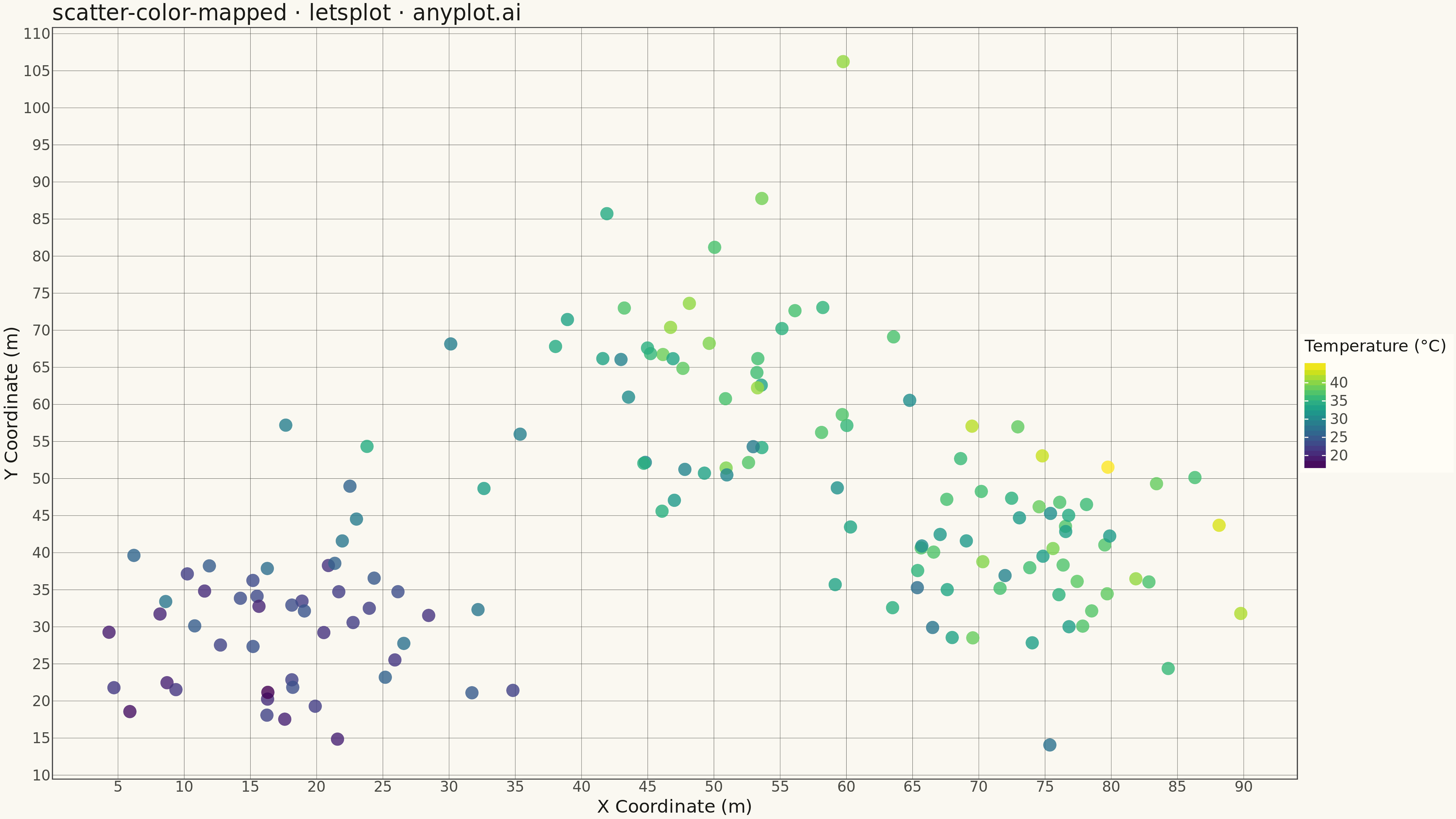
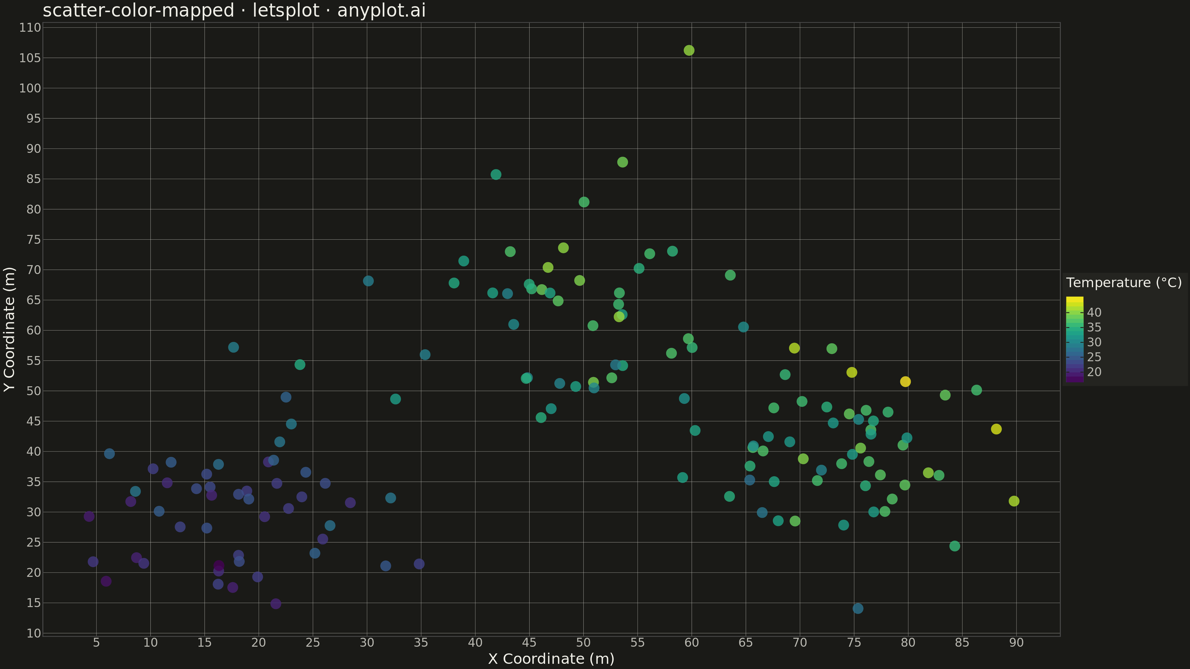
A scatter plot that encodes a third continuous variable using a colormap, allowing visualization of three dimensions on a 2D plane. This visualization is essential for exploring multivariate relationships where the third variable represents intensity, magnitude, or any continuous measurement. A colorbar provides a reference scale for interpreting the color values.
""" anyplot.ai
scatter-color-mapped: Color-Mapped Scatter Plot
Library: letsplot 4.9.0 | Python 3.13.13
Quality: 91/100 | Updated: 2026-05-08
"""

import os

import numpy as np
import pandas as pd
from lets_plot import *
from lets_plot import element_line, element_rect, element_text, theme
from lets_plot.export import ggsave as export_ggsave


LetsPlot.setup_html()

# Theme tokens (see prompts/default-style-guide.md "Theme-adaptive Chrome")
THEME = os.getenv("ANYPLOT_THEME", "light")
PAGE_BG = "#FAF8F1" if THEME == "light" else "#1A1A17"
ELEVATED_BG = "#FFFDF6" if THEME == "light" else "#242420"
INK = "#1A1A17" if THEME == "light" else "#F0EFE8"
INK_SOFT = "#4A4A44" if THEME == "light" else "#B8B7B0"

# Data - Simulating temperature readings across a spatial grid
np.random.seed(42)
n_points = 150

# Create spatial coordinates with some clustering
x = np.concatenate(
    [
        np.random.normal(20, 8, n_points // 3),
        np.random.normal(50, 10, n_points // 3),
        np.random.normal(75, 6, n_points - 2 * (n_points // 3)),
    ]
)
y = np.concatenate(
    [
        np.random.normal(30, 10, n_points // 3),
        np.random.normal(60, 12, n_points // 3),
        np.random.normal(40, 8, n_points - 2 * (n_points // 3)),
    ]
)

# Temperature as third variable - correlated with position
temperature = 15 + 0.2 * x + 0.15 * y + np.random.normal(0, 3, n_points)

df = pd.DataFrame({"x": x, "y": y, "temperature": temperature})

# Create the color-mapped scatter plot
anyplot_theme = theme(
    plot_background=element_rect(fill=PAGE_BG, color=PAGE_BG),
    panel_background=element_rect(fill=PAGE_BG),
    panel_grid_major=element_line(color=INK_SOFT, size=0.3, linetype="solid"),
    panel_grid_minor=element_blank(),
    axis_title=element_text(color=INK, size=20),
    axis_text=element_text(color=INK_SOFT, size=16),
    axis_line=element_line(color=INK_SOFT, size=0.5),
    plot_title=element_text(color=INK, size=24),
    legend_background=element_rect(fill=ELEVATED_BG, color=INK_SOFT),
    legend_text=element_text(color=INK_SOFT, size=16),
    legend_title=element_text(color=INK, size=18),
)

plot = (
    ggplot(df, aes(x="x", y="y", color="temperature"))
    + geom_point(
        size=6.5,
        alpha=0.8,
        tooltips=layer_tooltips()
        .line("X Coord|@x")
        .line("Y Coord|@y")
        .line("Temperature|@temperature"),
    )
    + scale_color_viridis(name="Temperature (°C)")
    + labs(
        x="X Coordinate (m)", y="Y Coordinate (m)", title="scatter-color-mapped · letsplot · anyplot.ai"
    )
    + theme_minimal()
    + anyplot_theme
    + ggsize(1600, 900)
)

# Save PNG (scale 3x to get 4800 × 2700 px)
export_ggsave(plot, filename=f"plot-{THEME}.png", path=".", scale=3)

# Save HTML for interactive version
export_ggsave(plot, filename=f"plot-{THEME}.html", path=".")
Runnable source as JSON, for any HTTP client: https://api.anyplot.ai/specs/scatter-color-mapped/letsplot/code. Any spec id and library id listed in llms-full.txt fit the same URL shape; every URL below is complete and callable.
{
  "spec_id": "scatter-color-mapped",
  "language": "python",
  "library": "letsplot",
  "page": "https://anyplot.ai/scatter-color-mapped/python/letsplot",
  "hub": "https://anyplot.ai/scatter-color-mapped",
  "code_json": "https://api.anyplot.ai/specs/scatter-color-mapped/letsplot/code",
  "spec_json": "https://api.anyplot.ai/specs/scatter-color-mapped",
  "render_light_png": "https://storage.googleapis.com/anyplot-images/plots/scatter-color-mapped/python/letsplot/plot-light.png",
  "render_dark_png": "https://storage.googleapis.com/anyplot-images/plots/scatter-color-mapped/python/letsplot/plot-dark.png",
  "interactive_light_html": "https://storage.googleapis.com/anyplot-images/plots/scatter-color-mapped/python/letsplot/plot-light.html",
  "interactive_dark_html": "https://storage.googleapis.com/anyplot-images/plots/scatter-color-mapped/python/letsplot/plot-dark.html",
  "quality_score": 91.0,
  "license": "MIT",
  "guide": "https://anyplot.ai/llms.txt"
}
Part of Color-Mapped Scatter Plot on anyplot.ai.