The same plot in 14 other libraries — JavaScript: Chart.js, Apache ECharts, Highcharts, MUI X Charts; Python: Altair, Bokeh, lets-plot, Matplotlib, Plotly, plotnine, Pygal, Seaborn; R: ggplot2; Julia: Makie.jl. Compare all 15 side by side: Complex Plane Visualization (Argand Diagram) in Python, R, Julia and JavaScript.
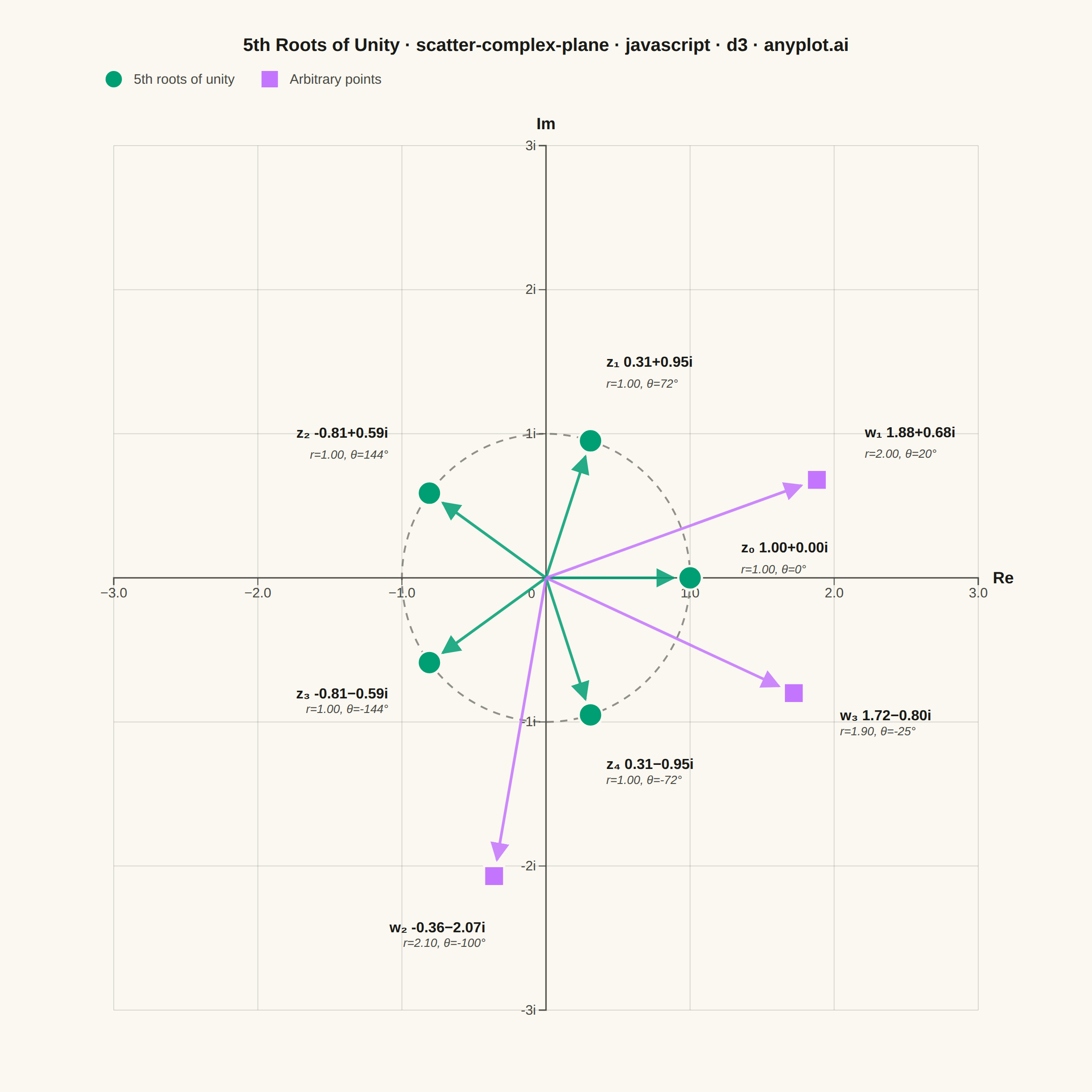
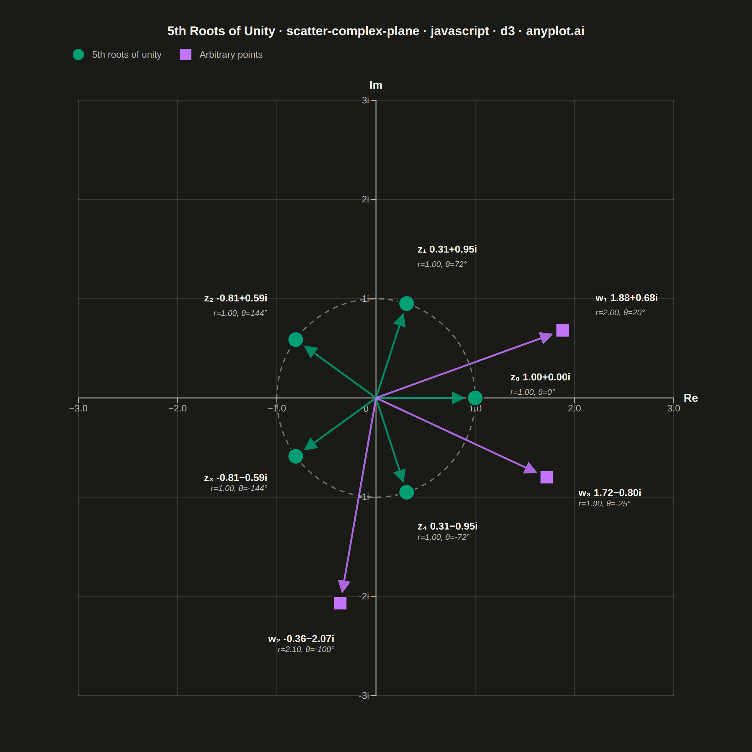
An Argand diagram plots complex numbers as points in the complex plane, with the real part on the x-axis and the imaginary part on the y-axis. Vectors from the origin to each point illustrate magnitude and phase angle, while a unit circle provides a geometric reference. This visualization is foundational for complex analysis, signal processing, and understanding operations like addition, multiplication, and roots of unity geometrically.
// anyplot.ai
// scatter-complex-plane: Complex Plane Visualization (Argand Diagram)
// Library: d3 7.9.0 | JavaScript 22.23.2
// Quality: 87/100 | Created: 2026-08-26
//# anyplot-orientation: square

const t = window.ANYPLOT_TOKENS;
const { width, height } = window.ANYPLOT_SIZE;

// --- Data (in-memory, deterministic) ----------------------------------------
// 5th roots of unity: z_k = e^(i*2*pi*k/5) — foundational for FFT / number theory,
// all sitting exactly on the unit circle by construction.
const subscripts = ["₀", "₁", "₂", "₃", "₄"];
const rootsOfUnity = d3.range(5).map((k) => {
  const theta = (2 * Math.PI * k) / 5;
  return {
    label: `z${subscripts[k]}`,
    re: Math.cos(theta),
    im: Math.sin(theta),
    category: "5th roots of unity",
  };
});

// A few arbitrary complex numbers, well outside the unit circle and spaced
// away from the roots' angles so vectors and annotations stay uncluttered
const arbitraryPoints = [
  { label: "w₁", re: 1.88, im: 0.68, category: "Arbitrary points" },
  { label: "w₂", re: -0.36, im: -2.07, category: "Arbitrary points" },
  { label: "w₃", re: 1.72, im: -0.8, category: "Arbitrary points" },
];

const points = [...rootsOfUnity, ...arbitraryPoints];

const categories = ["5th roots of unity", "Arbitrary points"];
const color = d3.scaleOrdinal().domain(categories).range([t.palette[0], t.palette[1]]);
const shapeOf = { "5th roots of unity": "circle", "Arbitrary points": "square" };

// --- Layout: force a true square plot area so the unit circle stays circular
const margin = { top: 160, right: 110, bottom: 90, left: 110 };
const availW = width - margin.left - margin.right;
const availH = height - margin.top - margin.bottom;
const side = Math.min(availW, availH);
const plotX = margin.left + (availW - side) / 2;
const plotY = margin.top + (availH - side) / 2;

const maxAbs = d3.max(points, (d) => Math.hypot(d.re, d.im));
const lim = Math.ceil(maxAbs * 1.35 * 2) / 2; // round outward to nearest 0.5
const gridTicks = d3.range(-Math.floor(lim), Math.floor(lim) + 1);

const xScale = d3.scaleLinear().domain([-lim, lim]).range([0, side]);
const yScale = d3.scaleLinear().domain([-lim, lim]).range([side, 0]);

const svg = d3.select("#container").append("svg").attr("width", width).attr("height", height);
const g = svg.append("g").attr("transform", `translate(${plotX},${plotY})`);

// --- Faint reference grid at integer real/imaginary values -------------------
for (const gt of gridTicks) {
  if (gt === 0) continue;
  g.append("line")
    .attr("x1", xScale(gt))
    .attr("x2", xScale(gt))
    .attr("y1", 0)
    .attr("y2", side)
    .attr("stroke", t.grid)
    .attr("stroke-width", 1);
  g.append("line")
    .attr("x1", 0)
    .attr("x2", side)
    .attr("y1", yScale(gt))
    .attr("y2", yScale(gt))
    .attr("stroke", t.grid)
    .attr("stroke-width", 1);
}

// --- Unit circle reference (dashed) -------------------------------------------
g.append("circle")
  .attr("cx", xScale(0))
  .attr("cy", yScale(0))
  .attr("r", xScale(1) - xScale(0))
  .attr("fill", "none")
  .attr("stroke", t.inkSoft)
  .attr("stroke-width", 2)
  .attr("stroke-dasharray", "8,7")
  .attr("opacity", 0.6);

// --- Real / imaginary axes through the origin, with labeled ticks ------------
const xAxis = g
  .append("g")
  .attr("transform", `translate(0,${yScale(0)})`)
  .call(
    d3
      .axisBottom(xScale)
      .tickValues(gridTicks.filter((v) => v !== 0))
      .tickSize(8)
  );
xAxis.selectAll("text").attr("fill", t.inkSoft).style("font-size", "15px");
xAxis.selectAll("line").attr("stroke", t.inkSoft);
xAxis.select(".domain").attr("stroke", t.inkSoft).attr("stroke-width", 1.5);

const yAxis = g
  .append("g")
  .attr("transform", `translate(${xScale(0)},0)`)
  .call(
    d3
      .axisLeft(yScale)
      .tickValues(gridTicks.filter((v) => v !== 0))
      .tickFormat((d) => `${d}i`)
      .tickSize(8)
  );
yAxis.selectAll("text").attr("fill", t.inkSoft).style("font-size", "15px");
yAxis.selectAll("line").attr("stroke", t.inkSoft);
yAxis.select(".domain").attr("stroke", t.inkSoft).attr("stroke-width", 1.5);

// Axis end labels + origin marker
g.append("text")
  .attr("x", side + 16)
  .attr("y", yScale(0) + 6)
  .attr("fill", t.ink)
  .style("font-size", "18px")
  .style("font-weight", "600")
  .text("Re");
g.append("text")
  .attr("x", xScale(0))
  .attr("y", -18)
  .attr("text-anchor", "middle")
  .attr("fill", t.ink)
  .style("font-size", "18px")
  .style("font-weight", "600")
  .text("Im");
g.append("text")
  .attr("x", xScale(0) - 12)
  .attr("y", yScale(0) + 22)
  .attr("text-anchor", "end")
  .attr("fill", t.inkSoft)
  .style("font-size", "14px")
  .text("0");

// --- Arrowhead marker defs (one per category color) ---------------------------
const defs = svg.append("defs");
categories.forEach((cat, i) => {
  defs
    .append("marker")
    .attr("id", `arrow-cat-${i}`)
    .attr("viewBox", "0 0 10 10")
    .attr("refX", 9)
    .attr("refY", 5)
    .attr("markerWidth", 7)
    .attr("markerHeight", 7)
    .attr("orient", "auto-start-reverse")
    .append("path")
    .attr("d", "M0,0 L10,5 L0,10 Z")
    .attr("fill", color(cat));
});

// --- Vectors from the origin to each complex number ---------------------------
const markerRadius = 13;
const ox = xScale(0);
const oy = yScale(0);

points.forEach((d) => {
  const px = xScale(d.re);
  const py = yScale(d.im);
  const dist = Math.hypot(px - ox, py - oy);
  const shrink = dist > 0 ? (dist - markerRadius - 5) / dist : 0;
  const catIndex = categories.indexOf(d.category);
  g.append("line")
    .attr("x1", ox)
    .attr("y1", oy)
    .attr("x2", ox + (px - ox) * shrink)
    .attr("y2", oy + (py - oy) * shrink)
    .attr("stroke", color(d.category))
    .attr("stroke-width", 3)
    .attr("opacity", 0.85)
    .attr("marker-end", `url(#arrow-cat-${catIndex})`);
});

// --- Points + rectangular/polar annotations ------------------------------------
const labelOffset = 56;
points.forEach((d) => {
  const px = xScale(d.re);
  const py = yScale(d.im);
  const dirLen = Math.hypot(px - ox, py - oy) || 1;
  const ux = (px - ox) / dirLen;
  const uy = (py - oy) / dirLen;

  const marker = g.append("g").attr("transform", `translate(${px},${py})`);
  if (shapeOf[d.category] === "circle") {
    marker
      .append("circle")
      .attr("r", markerRadius)
      .attr("fill", color(d.category))
      .attr("stroke", t.pageBg)
      .attr("stroke-width", 2.5);
  } else {
    const s = markerRadius * 1.7;
    marker
      .append("rect")
      .attr("x", -s / 2)
      .attr("y", -s / 2)
      .attr("width", s)
      .attr("height", s)
      .attr("fill", color(d.category))
      .attr("stroke", t.pageBg)
      .attr("stroke-width", 2.5);
  }

  const r = Math.hypot(d.re, d.im);
  const thetaDeg = (Math.atan2(d.im, d.re) * 180) / Math.PI;
  const sign = d.im >= 0 ? "+" : "−";
  const rectForm = `${d.label}  ${d.re.toFixed(2)}${sign}${Math.abs(d.im).toFixed(2)}i`;
  const polarForm = `r=${r.toFixed(2)}, θ=${thetaDeg.toFixed(0)}°`;
  const anchor = ux >= 0 ? "start" : "end";
  // Near-horizontal vectors (point sits close to the real axis) always go up:
  // the x-axis tick labels live in the band just below the axis, so a
  // downward annotation would crowd them (e.g. z0 lands on the "2.0" tick).
  const goesDown = Math.abs(uy) < 0.15 ? false : uy >= 0;

  const label = g
    .append("g")
    .attr("transform", `translate(${px + ux * labelOffset},${py + uy * labelOffset})`);
  label
    .append("text")
    .attr("text-anchor", anchor)
    .attr("dy", goesDown ? "0.4em" : "-1.75em")
    .attr("fill", t.ink)
    .style("font-size", "16px")
    .style("font-weight", "600")
    .text(rectForm);
  label
    .append("text")
    .attr("text-anchor", anchor)
    .attr("dy", goesDown ? "1.75em" : "-0.4em")
    .attr("fill", t.inkSoft)
    .style("font-size", "13px")
    .style("font-style", "italic")
    .text(polarForm);
});

// --- Legend --------------------------------------------------------------------
const legend = svg.append("g").attr("transform", `translate(${plotX},${margin.top - 68})`);
let legendX = 0;
categories.forEach((cat, i) => {
  const item = legend.append("g").attr("transform", `translate(${legendX},0)`);
  if (shapeOf[cat] === "circle") {
    item.append("circle").attr("r", 9).attr("cy", -5).attr("fill", color(cat));
  } else {
    item.append("rect").attr("x", -9).attr("y", -14).attr("width", 18).attr("height", 18).attr("fill", color(cat));
  }
  const label = item
    .append("text")
    .attr("x", 22)
    .attr("y", 0)
    .attr("fill", t.inkSoft)
    .style("font-size", "15px")
    .text(cat);
  legendX += label.node().getBBox().width + 60;
});

// --- Title -----------------------------------------------------------------
svg
  .append("text")
  .attr("x", width / 2)
  .attr("y", 56)
  .attr("text-anchor", "middle")
  .attr("fill", t.ink)
  .style("font-size", "20px")
  .style("font-weight", "600")
  .text("5th Roots of Unity · scatter-complex-plane · javascript · d3 · anyplot.ai");
Runnable source as JSON, for any HTTP client: https://api.anyplot.ai/specs/scatter-complex-plane/d3/code. Any spec id and library id listed in llms-full.txt fit the same URL shape; every URL below is complete and callable.
{
  "spec_id": "scatter-complex-plane",
  "language": "javascript",
  "library": "d3",
  "page": "https://anyplot.ai/scatter-complex-plane/javascript/d3",
  "hub": "https://anyplot.ai/scatter-complex-plane",
  "code_json": "https://api.anyplot.ai/specs/scatter-complex-plane/d3/code",
  "spec_json": "https://api.anyplot.ai/specs/scatter-complex-plane",
  "render_light_png": "https://storage.googleapis.com/anyplot-images/plots/scatter-complex-plane/javascript/d3/plot-light.png",
  "render_dark_png": "https://storage.googleapis.com/anyplot-images/plots/scatter-complex-plane/javascript/d3/plot-dark.png",
  "interactive_light_html": "https://storage.googleapis.com/anyplot-images/plots/scatter-complex-plane/javascript/d3/plot-light.html",
  "interactive_dark_html": "https://storage.googleapis.com/anyplot-images/plots/scatter-complex-plane/javascript/d3/plot-dark.html",
  "quality_score": 87.0,
  "license": "MIT",
  "guide": "https://anyplot.ai/llms.txt"
}
Part of Complex Plane Visualization (Argand Diagram) on anyplot.ai.