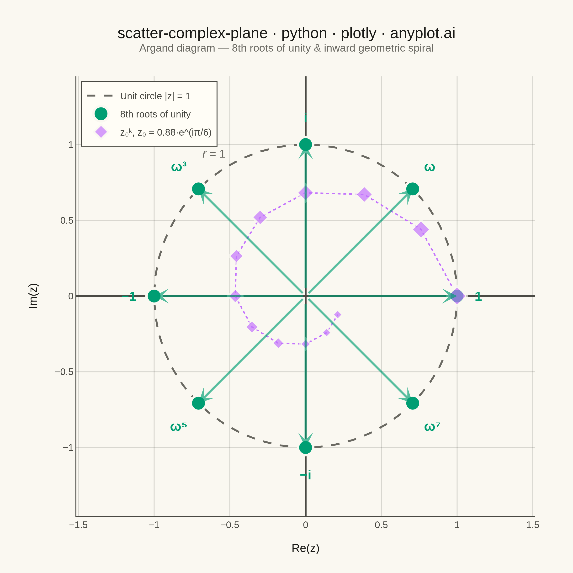
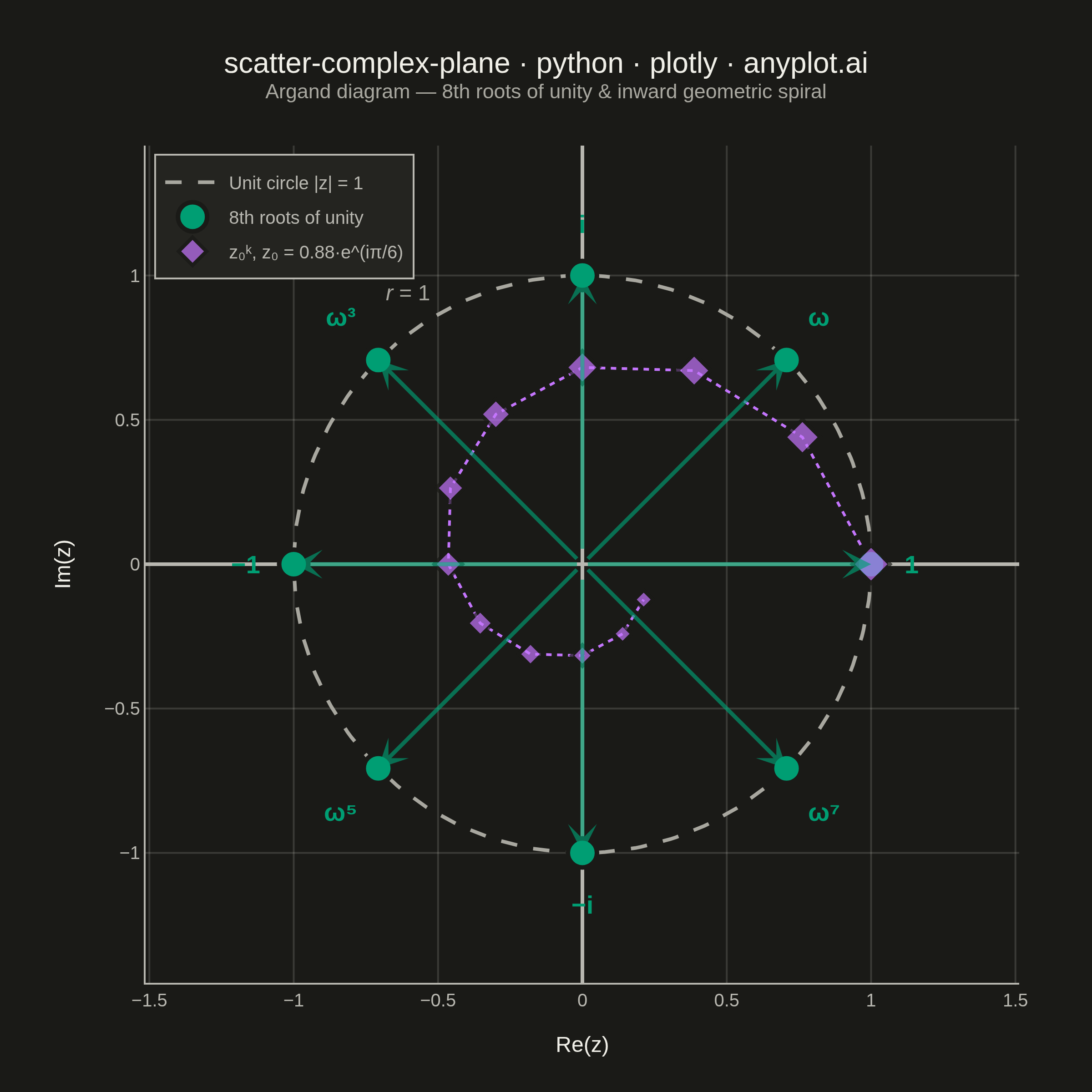
An Argand diagram plots complex numbers as points in the complex plane, with the real part on the x-axis and the imaginary part on the y-axis. Vectors from the origin to each point illustrate magnitude and phase angle, while a unit circle provides a geometric reference. This visualization is foundational for complex analysis, signal processing, and understanding operations like addition, multiplication, and roots of unity geometrically.
""" anyplot.ai
scatter-complex-plane: Complex Plane Visualization (Argand Diagram)
Library: plotly 6.7.0 | Python 3.13.13
Quality: 90/100 | Updated: 2026-06-02
"""
import os
import numpy as np
import plotly.graph_objects as go
# Theme tokens — Imprint palette chrome
THEME = os.getenv("ANYPLOT_THEME", "light")
PAGE_BG = "#FAF8F1" if THEME == "light" else "#1A1A17"
ELEVATED_BG = "#FFFDF6" if THEME == "light" else "#242420"
INK = "#1A1A17" if THEME == "light" else "#F0EFE8"
INK_SOFT = "#4A4A44" if THEME == "light" else "#B8B7B0"
INK_MUTED = "#6B6A63" if THEME == "light" else "#A8A79F"
GRID = "rgba(26,26,23,0.15)" if THEME == "light" else "rgba(240,239,232,0.15)"
# Imprint categorical palette — positions 1 and 2
C1 = "#009E73" # green — 8th roots of unity
C2 = "#C475FD" # purple — inward geometric spiral
# Data: 8th roots of unity ω = e^(2πi/8)
n_roots = 8
roots = [np.exp(2j * np.pi * k / n_roots) for k in range(n_roots)]
root_labels_display = ["1", "ω", "i", "ω³", "−1", "ω⁵", "−i", "ω⁷"]
root_labels_hover = [f"ω^{k}" for k in range(n_roots)]
# Data: geometric spiral — repeated multiplication by z₀ = 0.88·e^(iπ/6)
# Each step rotates 30° and contracts by factor 0.88; after 12 steps |z₀|¹² ≈ 0.20
z0 = 0.88 * np.exp(1j * np.pi / 6)
n_spiral = 12
spiral_pts = [z0**k for k in range(n_spiral)]
# Helper: text anchor relative to angle on unit circle
def root_anchor(k, n):
deg = 360 * k / n
if deg < 22.5 or deg >= 337.5:
return "left", 16, 0
elif deg < 67.5:
return "left", 10, 14
elif deg < 112.5:
return "center", 0, 18
elif deg < 157.5:
return "right", -10, 14
elif deg < 202.5:
return "right", -16, 0
elif deg < 247.5:
return "right", -10, -14
elif deg < 292.5:
return "center", 0, -18
else:
return "left", 10, -14
# Plot
fig = go.Figure()
# Unit circle reference (dashed)
theta_c = np.linspace(0, 2 * np.pi, 300)
fig.add_trace(
go.Scatter(
x=np.cos(theta_c).tolist(),
y=np.sin(theta_c).tolist(),
mode="lines",
line={"color": INK_MUTED, "width": 2, "dash": "dash"},
name="Unit circle |z| = 1",
hoverinfo="skip",
showlegend=True,
)
)
# Spiral connecting path (dotted)
fig.add_trace(
go.Scatter(
x=[z.real for z in spiral_pts],
y=[z.imag for z in spiral_pts],
mode="lines",
line={"color": C2, "width": 1.5, "dash": "dot"},
hoverinfo="skip",
showlegend=False,
)
)
# Vector arrows from origin to each 8th root
for pt in roots:
fig.add_annotation(
x=pt.real,
y=pt.imag,
ax=0,
ay=0,
xref="x",
yref="y",
axref="x",
ayref="y",
showarrow=True,
arrowhead=3,
arrowsize=1.2,
arrowwidth=2.2,
arrowcolor=C1,
opacity=0.65,
)
# Root label annotations
for k, (pt, label) in enumerate(zip(roots, root_labels_display, strict=True)):
xa, xs, ys = root_anchor(k, n_roots)
ya = "middle"
if ys > 0:
ya = "bottom"
elif ys < 0:
ya = "top"
fig.add_annotation(
x=pt.real,
y=pt.imag,
text=f"<b>{label}</b>",
showarrow=False,
font={"size": 14, "color": C1},
xanchor=xa,
yanchor=ya,
xshift=xs,
yshift=ys,
)
# Scatter trace: 8th roots of unity
fig.add_trace(
go.Scatter(
x=[z.real for z in roots],
y=[z.imag for z in roots],
mode="markers",
marker={"size": 16, "color": C1, "line": {"color": PAGE_BG, "width": 2.5}, "symbol": "circle"},
name="8th roots of unity",
customdata=[[root_labels_hover[k], abs(roots[k]), np.degrees(np.angle(roots[k]))] for k in range(n_roots)],
hovertemplate=(
"<b>%{customdata[0]}</b><br>"
"Re: %{x:.4f}<br>Im: %{y:.4f}<br>"
"|z| = %{customdata[1]:.4f}<br>"
"arg(z) = %{customdata[2]:.1f}°"
"<extra>8th roots of unity</extra>"
),
)
)
# Scatter trace: geometric spiral (marker size decreases to show convergence)
spiral_sizes = [max(7, round(16 - k * 0.75)) for k in range(n_spiral)]
fig.add_trace(
go.Scatter(
x=[z.real for z in spiral_pts],
y=[z.imag for z in spiral_pts],
mode="markers",
marker={"size": spiral_sizes, "color": C2, "line": {"color": PAGE_BG, "width": 2}, "symbol": "diamond"},
name="z₀ᵏ, z₀ = 0.88·e^(iπ/6)",
customdata=[[k, abs(spiral_pts[k]), np.degrees(np.angle(spiral_pts[k]))] for k in range(n_spiral)],
hovertemplate=(
"<b>z₀^%{customdata[0]}</b><br>"
"Re: %{x:.4f}<br>Im: %{y:.4f}<br>"
"|z₀ᵏ| = %{customdata[1]:.4f}<br>"
"arg = %{customdata[2]:.1f}°"
"<extra>Geometric spiral</extra>"
),
)
)
# "r = 1" label at 120° on unit circle — clear of all data
fig.add_annotation(
x=np.cos(np.radians(120)),
y=np.sin(np.radians(120)),
text="<i>r</i> = 1",
showarrow=False,
font={"size": 12, "color": INK_MUTED},
xshift=-16,
yshift=12,
)
# Title — compute font size from character count
title_str = "scatter-complex-plane · python · plotly · anyplot.ai"
n_chars = len(title_str)
default_fs = 16
title_fs = max(11, round(default_fs * 67 / n_chars)) if n_chars > 67 else default_fs
fig.update_layout(
autosize=False,
title={
"text": (
f"{title_str}<br>"
f"<sup style='color:{INK_MUTED}; font-weight:normal'>"
"Argand diagram — 8th roots of unity & inward geometric spiral"
"</sup>"
),
"font": {"size": title_fs, "color": INK},
"x": 0.5,
"xanchor": "center",
},
xaxis={
"title": {"text": "Re(z)", "font": {"size": 12, "color": INK}},
"tickfont": {"size": 10, "color": INK_SOFT},
"zeroline": True,
"zerolinewidth": 2,
"zerolinecolor": INK_SOFT,
"gridcolor": GRID,
"linecolor": INK_SOFT,
"showgrid": True,
"dtick": 0.5,
"range": [-1.45, 1.45],
},
yaxis={
"title": {"text": "Im(z)", "font": {"size": 12, "color": INK}},
"tickfont": {"size": 10, "color": INK_SOFT},
"zeroline": True,
"zerolinewidth": 2,
"zerolinecolor": INK_SOFT,
"gridcolor": GRID,
"linecolor": INK_SOFT,
"showgrid": True,
"scaleanchor": "x",
"scaleratio": 1,
"dtick": 0.5,
"range": [-1.45, 1.45],
},
paper_bgcolor=PAGE_BG,
plot_bgcolor=PAGE_BG,
font={"color": INK},
legend={
"font": {"size": 10, "color": INK_SOFT},
"bgcolor": ELEVATED_BG,
"bordercolor": INK_SOFT,
"borderwidth": 1,
"x": 0.01,
"y": 0.99,
"xanchor": "left",
"yanchor": "top",
},
margin={"l": 80, "r": 40, "t": 80, "b": 60},
)
# Save — square canvas: 600×600 × scale=4 → 2400×2400 px
fig.write_image(f"plot-{THEME}.png", width=600, height=600, scale=4)
fig.write_html(f"plot-{THEME}.html", include_plotlyjs="cdn")
Runnable source as JSON, for any HTTP client: https://api.anyplot.ai/specs/scatter-complex-plane/plotly/code. Any spec id and library id listed in llms-full.txt fit the same URL shape; every URL below is complete and callable.
{
  "spec_id": "scatter-complex-plane",
  "language": "python",
  "library": "plotly",
  "page": "https://anyplot.ai/scatter-complex-plane/python/plotly",
  "hub": "https://anyplot.ai/scatter-complex-plane",
  "code_json": "https://api.anyplot.ai/specs/scatter-complex-plane/plotly/code",
  "spec_json": "https://api.anyplot.ai/specs/scatter-complex-plane",
  "render_light_png": "https://storage.googleapis.com/anyplot-images/plots/scatter-complex-plane/python/plotly/plot-light.png",
  "render_dark_png": "https://storage.googleapis.com/anyplot-images/plots/scatter-complex-plane/python/plotly/plot-dark.png",
  "interactive_light_html": "https://storage.googleapis.com/anyplot-images/plots/scatter-complex-plane/python/plotly/plot-light.html",
  "interactive_dark_html": "https://storage.googleapis.com/anyplot-images/plots/scatter-complex-plane/python/plotly/plot-dark.html",
  "quality_score": 90.0,
  "license": "MIT",
  "guide": "https://anyplot.ai/llms.txt"
}
Part of Complex Plane Visualization (Argand Diagram) on anyplot.ai.