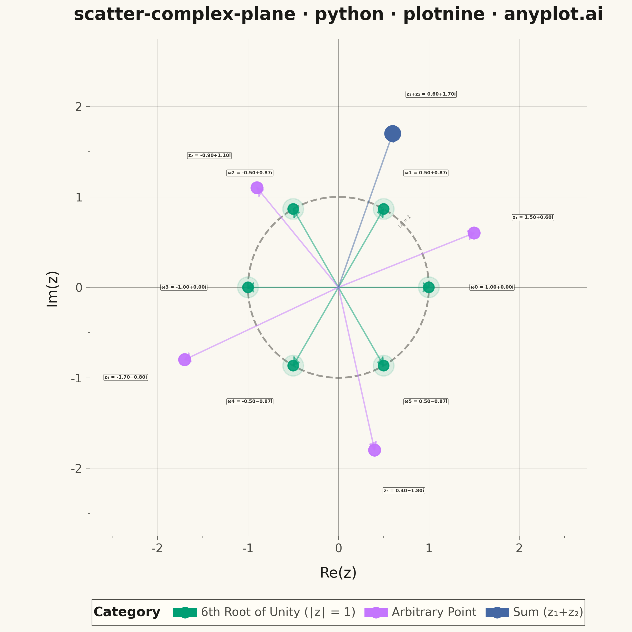
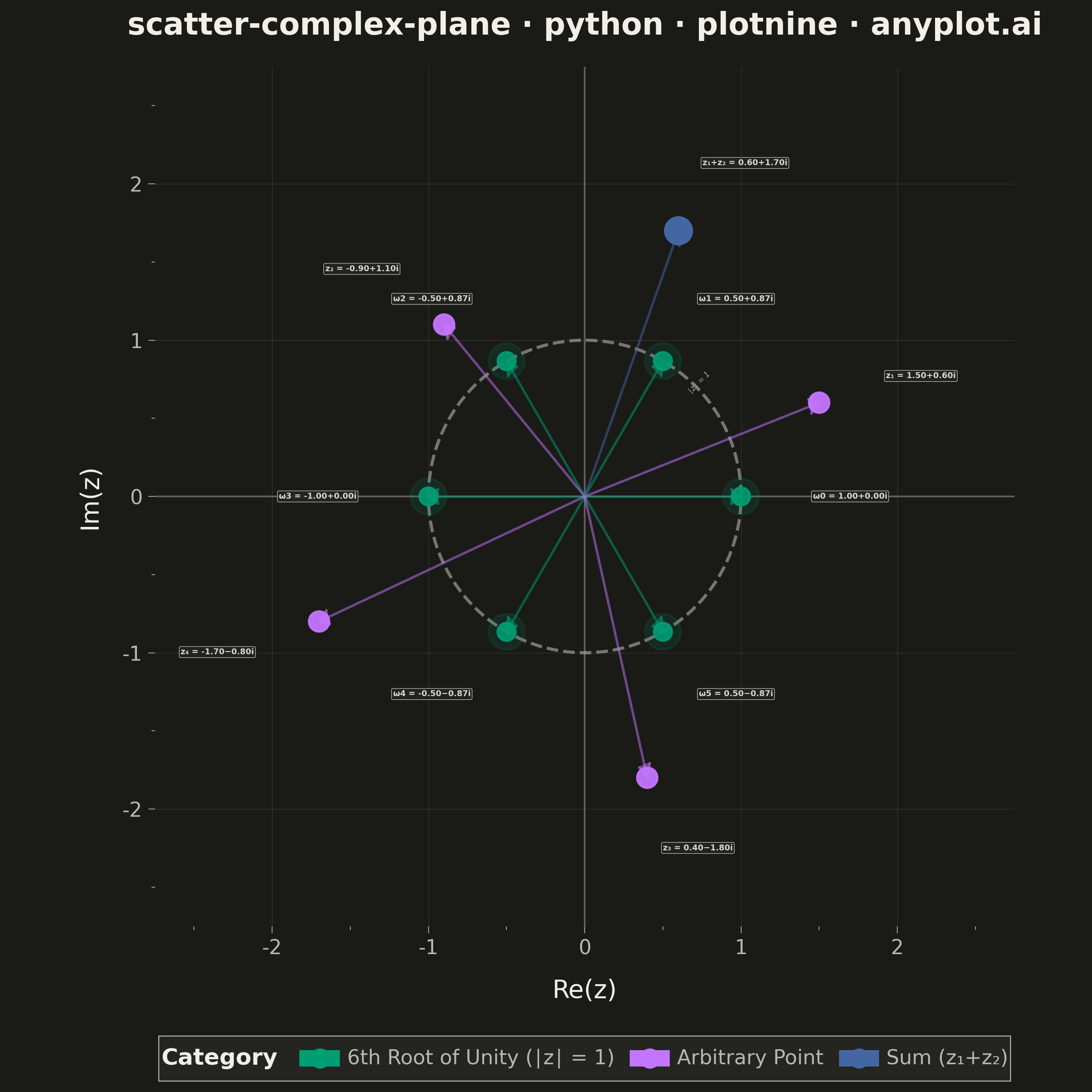
An Argand diagram plots complex numbers as points in the complex plane, with the real part on the x-axis and the imaginary part on the y-axis. Vectors from the origin to each point illustrate magnitude and phase angle, while a unit circle provides a geometric reference. This visualization is foundational for complex analysis, signal processing, and understanding operations like addition, multiplication, and roots of unity geometrically.
""" anyplot.ai
scatter-complex-plane: Complex Plane Visualization (Argand Diagram)
Library: plotnine 0.15.4 | Python 3.13.13
Quality: 88/100 | Updated: 2026-06-02
"""

import os

import numpy as np
import pandas as pd
from plotnine import (
    aes,
    annotate,
    arrow,
    coord_fixed,
    element_blank,
    element_line,
    element_rect,
    element_text,
    geom_hline,
    geom_label,
    geom_path,
    geom_point,
    geom_segment,
    geom_vline,
    ggplot,
    guide_legend,
    guides,
    labs,
    scale_alpha_identity,
    scale_color_manual,
    scale_size_identity,
    scale_x_continuous,
    scale_y_continuous,
    theme,
    theme_minimal,
)


# Theme-adaptive chrome tokens
THEME = os.getenv("ANYPLOT_THEME", "light")
PAGE_BG = "#FAF8F1" if THEME == "light" else "#1A1A17"
ELEVATED_BG = "#FFFDF6" if THEME == "light" else "#242420"
INK = "#1A1A17" if THEME == "light" else "#F0EFE8"
INK_SOFT = "#4A4A44" if THEME == "light" else "#B8B7B0"
INK_MUTED = "#6B6A63" if THEME == "light" else "#A8A79F"

# Imprint categorical palette — 8 hues, hybrid-v3 sort
IMPRINT_PALETTE = ["#009E73", "#C475FD", "#4467A3", "#BD8233", "#AE3030", "#2ABCCD", "#954477", "#99B314"]
color_roots = IMPRINT_PALETTE[0]  # brand green — 6th roots of unity
color_arb = IMPRINT_PALETTE[1]  # lavender — arbitrary points
color_sum = IMPRINT_PALETTE[2]  # blue — complex sum

# Data — 6th roots of unity (evenly spaced at 60° intervals on unit circle)
n_roots = 6
angles_roots = np.array([2 * np.pi * k / n_roots for k in range(n_roots)])
roots_real = np.cos(angles_roots)
roots_imag = np.sin(angles_roots)
roots_labels = [f"ω{k}" for k in range(n_roots)]

# Arbitrary points spread across all four quadrants
arbitrary_real = np.array([1.5, -0.9, 0.4, -1.7])
arbitrary_imag = np.array([0.6, 1.1, -1.8, -0.8])
arbitrary_labels = ["z₁", "z₂", "z₃", "z₄"]

# Complex addition: z₁ + z₂ — resultant vector only, no parallelogram construction lines
sum_real = arbitrary_real[0] + arbitrary_real[1]  # 0.6
sum_imag = arbitrary_imag[0] + arbitrary_imag[1]  # 1.7

real = np.concatenate([roots_real, arbitrary_real, [sum_real]])
imag = np.concatenate([roots_imag, arbitrary_imag, [sum_imag]])
labels = roots_labels + arbitrary_labels + ["z₁+z₂"]
category = ["6th Root of Unity"] * n_roots + ["Arbitrary Point"] * len(arbitrary_real) + ["Sum (z₁+z₂)"]

df_points = pd.DataFrame({"real": real, "imag": imag, "label": labels, "category": category})

# Annotation text: point name + rectangular form (a+bi)
annotations = []
for r, i, lbl in zip(real, imag, labels, strict=True):
    sign = "+" if i >= 0 else "−"
    annotations.append(f"{lbl} = {r:.2f}{sign}{abs(i):.2f}i")
df_points["annotation"] = annotations

# Vectors from origin to each point
df_vectors = pd.DataFrame(
    {"x": [0.0] * len(real), "y": [0.0] * len(real), "xend": real, "yend": imag, "category": category}
)

# Unit circle reference
theta = np.linspace(0, 2 * np.pi, 300)
df_circle = pd.DataFrame({"x": np.cos(theta), "y": np.sin(theta)})

# Radial label offsets — spread labels away from vectors to reduce crowding
angles = np.arctan2(imag, real)
label_radius = 0.46
x_offsets = label_radius * np.cos(angles)
y_offsets = label_radius * np.sin(angles)
ha_values = ["left" if np.cos(a) >= 0 else "right" for a in angles]

df_labels = pd.DataFrame({"x": real + x_offsets, "y": imag + y_offsets, "annotation": annotations, "ha": ha_values})

# Visual hierarchy via point size (few data points → prominent markers)
df_points["pt_size"] = [3.5] * n_roots + [4.0] * len(arbitrary_real) + [5.5]
df_points["pt_alpha"] = [0.90] * n_roots + [0.95] * len(arbitrary_real) + [1.0]

colors = [color_roots, color_arb, color_sum]

plot = (
    ggplot()
    # Reference axes through origin
    + geom_hline(yintercept=0, color=INK_SOFT, size=0.4, linetype="solid", alpha=0.4)
    + geom_vline(xintercept=0, color=INK_SOFT, size=0.4, linetype="solid", alpha=0.4)
    # Unit circle — dashed reference
    + geom_path(df_circle, aes(x="x", y="y"), color=INK_MUTED, linetype="dashed", size=0.7, alpha=0.65)
    + annotate("text", x=0.62, y=0.80, label="∣z∣ = 1", size=3.8, color=INK_MUTED, fontstyle="italic", angle=50)
    # Vectors from origin (no parallelogram construction lines)
    + geom_segment(
        df_vectors,
        aes(x="x", y="y", xend="xend", yend="yend", color="category"),
        size=0.55,
        alpha=0.50,
        arrow=arrow(length=0.09, type="closed"),
    )
    # Points — main scatter layer with visual hierarchy
    + geom_point(df_points, aes(x="real", y="imag", color="category", size="pt_size", alpha="pt_alpha"))
    + scale_size_identity()
    + scale_alpha_identity()
    # Halo ring on roots of unity for emphasis
    + geom_point(
        df_points[df_points["category"] == "6th Root of Unity"],
        aes(x="real", y="imag"),
        size=7.5,
        color=color_roots,
        alpha=0.12,
    )
    # Annotation labels — split by horizontal alignment (plotnine limitation)
    + geom_label(
        df_labels[df_labels["ha"] == "left"],
        aes(x="x", y="y", label="annotation"),
        size=3.8,
        color=INK,
        fill=ELEVATED_BG,
        alpha=0.88,
        ha="left",
        fontweight="bold",
        label_padding=0.18,
        label_size=0.2,
        boxstyle="round,pad=0.2",
    )
    + geom_label(
        df_labels[df_labels["ha"] == "right"],
        aes(x="x", y="y", label="annotation"),
        size=3.8,
        color=INK,
        fill=ELEVATED_BG,
        alpha=0.88,
        ha="right",
        fontweight="bold",
        label_padding=0.18,
        label_size=0.2,
        boxstyle="round,pad=0.2",
    )
    + labs(x="Re(z)", y="Im(z)", title="scatter-complex-plane · python · plotnine · anyplot.ai", color="Category")
    + scale_x_continuous(limits=(-2.5, 2.5), breaks=[-2, -1, 0, 1, 2])
    + scale_y_continuous(limits=(-2.5, 2.5), breaks=[-2, -1, 0, 1, 2])
    + coord_fixed(ratio=1)
    + scale_color_manual(values=colors, labels=["6th Root of Unity (∣z∣ = 1)", "Arbitrary Point", "Sum (z₁+z₂)"])
    + guides(color=guide_legend(override_aes={"size": 3.5, "alpha": 1.0}))
    + theme_minimal()
    + theme(
        figure_size=(6, 6),
        text=element_text(family="sans-serif", size=7, color=INK),
        plot_title=element_text(size=12, weight="bold", color=INK, margin={"b": 10}),
        axis_title_x=element_text(size=10, color=INK, margin={"t": 8}),
        axis_title_y=element_text(size=10, color=INK, margin={"r": 8}),
        axis_text=element_text(size=8, color=INK_SOFT),
        axis_ticks=element_line(color=INK_SOFT, size=0.3),
        legend_text=element_text(size=8, color=INK_SOFT),
        legend_title=element_text(size=9, weight="bold", color=INK),
        legend_position="bottom",
        legend_background=element_rect(fill=ELEVATED_BG, color=INK_SOFT, size=0.4),
        legend_key=element_rect(fill="none", color="none"),
        panel_background=element_rect(fill=PAGE_BG, color="none"),
        plot_background=element_rect(fill=PAGE_BG, color=PAGE_BG),
        panel_grid_major=element_line(color=INK, size=0.2, alpha=0.15),
        panel_grid_minor=element_blank(),
        panel_border=element_blank(),
    )
)

plot.save(f"plot-{THEME}.png", dpi=400, width=6, height=6, units="in", verbose=False)
Runnable source as JSON, for any HTTP client: https://api.anyplot.ai/specs/scatter-complex-plane/plotnine/code. Any spec id and library id listed in llms-full.txt fit the same URL shape; every URL below is complete and callable.
{
  "spec_id": "scatter-complex-plane",
  "language": "python",
  "library": "plotnine",
  "page": "https://anyplot.ai/scatter-complex-plane/python/plotnine",
  "hub": "https://anyplot.ai/scatter-complex-plane",
  "code_json": "https://api.anyplot.ai/specs/scatter-complex-plane/plotnine/code",
  "spec_json": "https://api.anyplot.ai/specs/scatter-complex-plane",
  "render_light_png": "https://storage.googleapis.com/anyplot-images/plots/scatter-complex-plane/python/plotnine/plot-light.png",
  "render_dark_png": "https://storage.googleapis.com/anyplot-images/plots/scatter-complex-plane/python/plotnine/plot-dark.png",
  "quality_score": 88.0,
  "license": "MIT",
  "guide": "https://anyplot.ai/llms.txt"
}
Part of Complex Plane Visualization (Argand Diagram) on anyplot.ai.