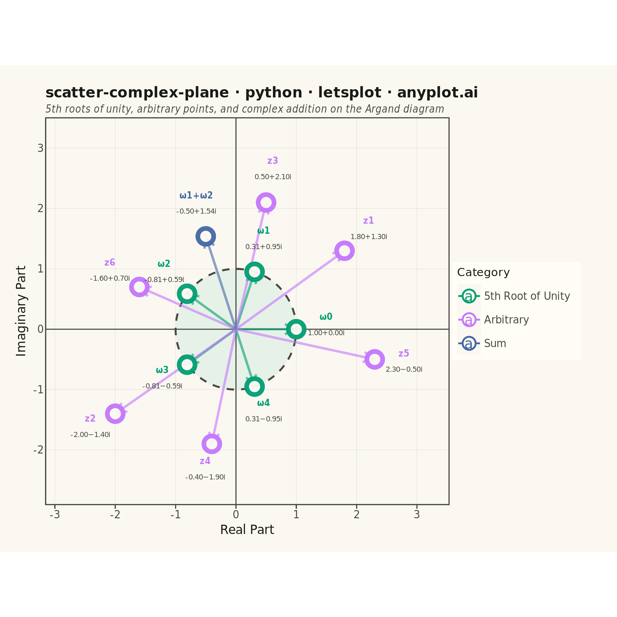
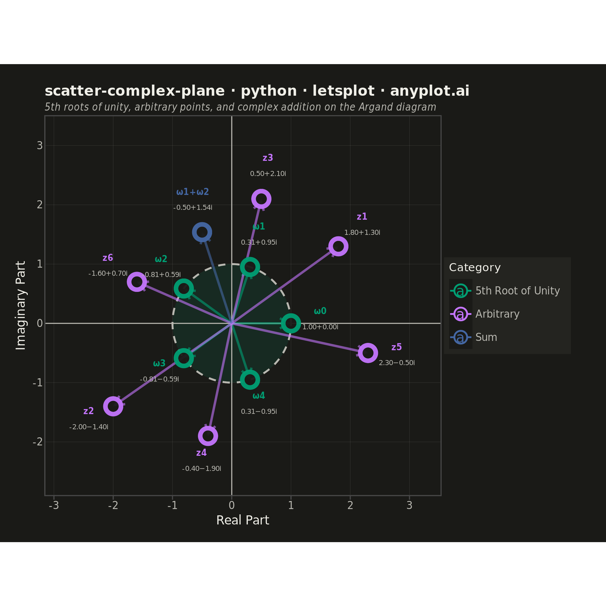
An Argand diagram plots complex numbers as points in the complex plane, with the real part on the x-axis and the imaginary part on the y-axis. Vectors from the origin to each point illustrate magnitude and phase angle, while a unit circle provides a geometric reference. This visualization is foundational for complex analysis, signal processing, and understanding operations like addition, multiplication, and roots of unity geometrically.
""" anyplot.ai
scatter-complex-plane: Complex Plane Visualization (Argand Diagram)
Library: letsplot 4.10.1 | Python 3.13.13
Quality: 87/100 | Updated: 2026-06-02
"""

import os

import numpy as np
import pandas as pd
from lets_plot import *
from lets_plot.export import ggsave as export_ggsave


LetsPlot.setup_html()

THEME = os.getenv("ANYPLOT_THEME", "light")

# Imprint palette — theme-independent, canonical order
IMPRINT_PALETTE = ["#009E73", "#C475FD", "#4467A3", "#BD8233", "#AE3030", "#2ABCCD", "#954477", "#99B314"]

# Theme-adaptive chrome tokens
PAGE_BG = "#FAF8F1" if THEME == "light" else "#1A1A17"
ELEVATED_BG = "#FFFDF6" if THEME == "light" else "#242420"
INK = "#1A1A17" if THEME == "light" else "#F0EFE8"
INK_SOFT = "#4A4A44" if THEME == "light" else "#B8B7B0"
INK_MUTED = "#6B6A63" if THEME == "light" else "#A8A79F"
RULE = "rgba(26,26,23,0.15)" if THEME == "light" else "rgba(240,239,232,0.15)"

# Unit circle subtle tint using Imprint brand green
CIRCLE_ALPHA = 0.08 if THEME == "light" else 0.12

# Data — 5th roots of unity + arbitrary points + complex sum
np.random.seed(42)

n_roots = 5
roots_angles = np.array([2 * np.pi * k / n_roots for k in range(n_roots)])
roots_real = np.cos(roots_angles)
roots_imag = np.sin(roots_angles)
roots_labels = [f"ω{k}" for k in range(n_roots)]

arbitrary_real = np.array([1.8, -2.0, 0.5, -0.4, 2.3, -1.6])
arbitrary_imag = np.array([1.3, -1.4, 2.1, -1.9, -0.5, 0.7])
arbitrary_labels = [f"z{i + 1}" for i in range(len(arbitrary_real))]

sum_real = np.array([roots_real[1] + roots_real[2]])
sum_imag = np.array([roots_imag[1] + roots_imag[2]])
sum_labels = ["ω1+ω2"]

all_real = np.concatenate([roots_real, arbitrary_real, sum_real])
all_imag = np.concatenate([roots_imag, arbitrary_imag, sum_imag])
all_labels = roots_labels + arbitrary_labels + sum_labels
all_category = ["5th Root of Unity"] * n_roots + ["Arbitrary"] * len(arbitrary_real) + ["Sum"]

all_mag = np.sqrt(all_real**2 + all_imag**2)
all_angle_deg = np.degrees(np.arctan2(all_imag, all_real))

rect_labels = []
for r, i in zip(all_real, all_imag, strict=True):
    sign = "+" if i >= 0 else "−"
    rect_labels.append(f"{r:.2f}{sign}{abs(i):.2f}i")

polar_labels = []
for mag, ang in zip(all_mag, all_angle_deg, strict=True):
    polar_labels.append(f"r={mag:.2f}, θ={ang:.0f}°")

df = pd.DataFrame(
    {
        "real": all_real,
        "imaginary": all_imag,
        "label": all_labels,
        "category": all_category,
        "rect_form": rect_labels,
        "polar_form": polar_labels,
        "magnitude": all_mag,
        "angle_deg": all_angle_deg,
    }
)

# Radial label placement with iterative repulsion to reduce overlap
angles = np.arctan2(all_imag, all_real)
base_offset = 0.5
label_x = all_real + base_offset * np.cos(angles)
label_y = all_imag + base_offset * np.sin(angles) + 0.2

min_sep = 0.9
for _ in range(20):
    for i in range(len(label_x)):
        for j in range(i + 1, len(label_x)):
            dx = label_x[i] - label_x[j]
            dy = label_y[i] - label_y[j]
            dist = np.sqrt(dx**2 + dy**2)
            if dist < min_sep:
                push = 0.15 * (min_sep - dist) / max(dist, 0.01)
                label_x[i] += dx * push
                label_y[i] += dy * push
                label_x[j] -= dx * push
                label_y[j] -= dy * push

df["label_x"] = label_x
df["label_y"] = label_y

# Vectors from origin to each point
arrows_df = pd.DataFrame(
    {
        "x_start": np.zeros(len(all_real)),
        "y_start": np.zeros(len(all_real)),
        "x_end": all_real,
        "y_end": all_imag,
        "category": all_category,
    }
)

# Unit circle path
theta = np.linspace(0, 2 * np.pi, 200)
circle_df = pd.DataFrame({"x": np.cos(theta), "y": np.sin(theta)})

# 3 categories use Imprint positions 1–3
colors = IMPRINT_PALETTE[:3]

# Tooltips for HTML interactivity — lets-plot distinctive feature
point_tooltips = (
    layer_tooltips()
    .title("@label")
    .line("Category|@category")
    .line("Rectangular|@rect_form")
    .line("Polar|@polar_form")
    .format("magnitude", ".3f")
    .format("angle_deg", ".1f")
)

anyplot_theme = theme(
    plot_background=element_rect(fill=PAGE_BG, color=PAGE_BG),
    panel_background=element_rect(fill=PAGE_BG),
    panel_grid_major=element_line(color=RULE, size=0.25),
    panel_grid_minor=element_blank(),
    axis_title=element_text(size=12, color=INK),
    axis_text=element_text(size=10, color=INK_SOFT),
    axis_line=element_blank(),
    panel_border=element_blank(),
    plot_title=element_text(size=14, color=INK, face="bold"),
    plot_subtitle=element_text(size=10, color=INK_SOFT, face="italic"),
    legend_background=element_rect(fill=ELEVATED_BG, color=INK_SOFT),
    legend_text=element_text(size=10, color=INK_SOFT),
    legend_title=element_text(size=11, color=INK),
    plot_margin=[20, 35, 15, 15],
)

plot = (
    ggplot()
    # Unit circle filled region (subtle Imprint green tint)
    + geom_polygon(
        data=circle_df,
        mapping=aes(x="x", y="y"),
        fill=IMPRINT_PALETTE[0],
        alpha=CIRCLE_ALPHA,
        color="rgba(0,0,0,0)",
    )
    # Dashed unit circle reference
    + geom_path(
        data=circle_df,
        mapping=aes(x="x", y="y"),
        color=INK_SOFT,
        size=0.8,
        linetype="dashed",
    )
    # Real and imaginary axes through origin
    + geom_hline(yintercept=0, color=INK_SOFT, size=0.4)
    + geom_vline(xintercept=0, color=INK_SOFT, size=0.4)
    # Vectors from origin (magnitude and phase visualization)
    + geom_segment(
        data=arrows_df,
        mapping=aes(
            x="x_start", y="y_start", xend="x_end", yend="y_end", color="category"
        ),
        size=1.0,
        alpha=0.6,
        arrow=arrow(length=10, type="open"),
    )
    # Points with interactive tooltips
    + geom_point(
        data=df,
        mapping=aes(x="real", y="imaginary", color="category"),
        size=5,
        alpha=0.95,
        shape=21,
        fill=PAGE_BG,
        stroke=2.0,
        tooltips=point_tooltips,
    )
    # Bold name labels positioned radially outward
    + geom_text(
        data=df,
        mapping=aes(x="label_x", y="label_y", label="label", color="category"),
        size=4,
        fontface="bold",
    )
    # Rectangular form (a+bi) below name
    + geom_text(
        data=df,
        mapping=aes(x="label_x", y="label_y", label="rect_form"),
        size=3.5,
        color=INK_SOFT,
        nudge_y=-0.26,
    )
    + scale_color_manual(values=colors)
    + coord_fixed()
    + labs(
        x="Real Part",
        y="Imaginary Part",
        title="scatter-complex-plane · python · letsplot · anyplot.ai",
        subtitle="5th roots of unity, arbitrary points, and complex addition on the Argand diagram",
        color="Category",
    )
    + scale_x_continuous(breaks=[-3, -2, -1, 0, 1, 2, 3], expand=[0.12, 0.12])
    + scale_y_continuous(breaks=[-3, -2, -1, 0, 1, 2, 3], expand=[0.12, 0.12])
    # Square canvas: 600×600 × scale=4 → 2400×2400 px (equal-aspect complex plane)
    + ggsize(600, 600)
    + anyplot_theme
)

# Save PNG (scale=4 → 2400×2400 px) and interactive HTML to current directory
export_ggsave(plot, filename=f"plot-{THEME}.png", path=".", scale=4)
export_ggsave(plot, filename=f"plot-{THEME}.html", path=".")
Runnable source as JSON, for any HTTP client: https://api.anyplot.ai/specs/scatter-complex-plane/letsplot/code. Any spec id and library id listed in llms-full.txt fit the same URL shape; every URL below is complete and callable.
{
  "spec_id": "scatter-complex-plane",
  "language": "python",
  "library": "letsplot",
  "page": "https://anyplot.ai/scatter-complex-plane/python/letsplot",
  "hub": "https://anyplot.ai/scatter-complex-plane",
  "code_json": "https://api.anyplot.ai/specs/scatter-complex-plane/letsplot/code",
  "spec_json": "https://api.anyplot.ai/specs/scatter-complex-plane",
  "render_light_png": "https://storage.googleapis.com/anyplot-images/plots/scatter-complex-plane/python/letsplot/plot-light.png",
  "render_dark_png": "https://storage.googleapis.com/anyplot-images/plots/scatter-complex-plane/python/letsplot/plot-dark.png",
  "interactive_light_html": "https://storage.googleapis.com/anyplot-images/plots/scatter-complex-plane/python/letsplot/plot-light.html",
  "interactive_dark_html": "https://storage.googleapis.com/anyplot-images/plots/scatter-complex-plane/python/letsplot/plot-dark.html",
  "quality_score": 87.0,
  "license": "MIT",
  "guide": "https://anyplot.ai/llms.txt"
}
Part of Complex Plane Visualization (Argand Diagram) on anyplot.ai.