The same plot in 14 other libraries — JavaScript: Chart.js, Apache ECharts, Highcharts, MUI X Charts; Python: Altair, Bokeh, lets-plot, Matplotlib, Plotly, plotnine, Pygal, Seaborn; R: ggplot2; Julia: Makie.jl. Compare all 15 side by side: Frequency Spectrum Plot in Python, R, Julia and JavaScript.
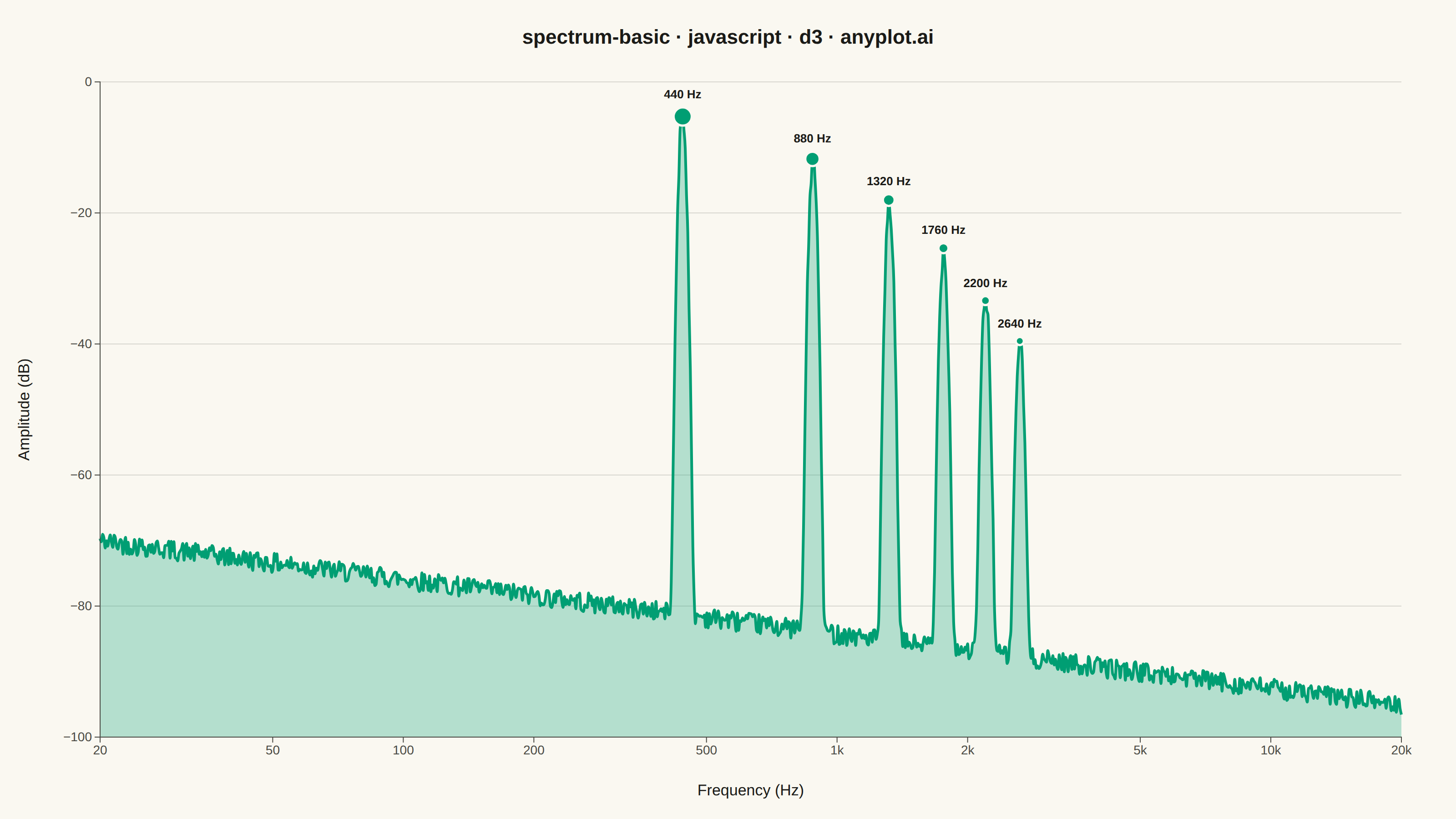
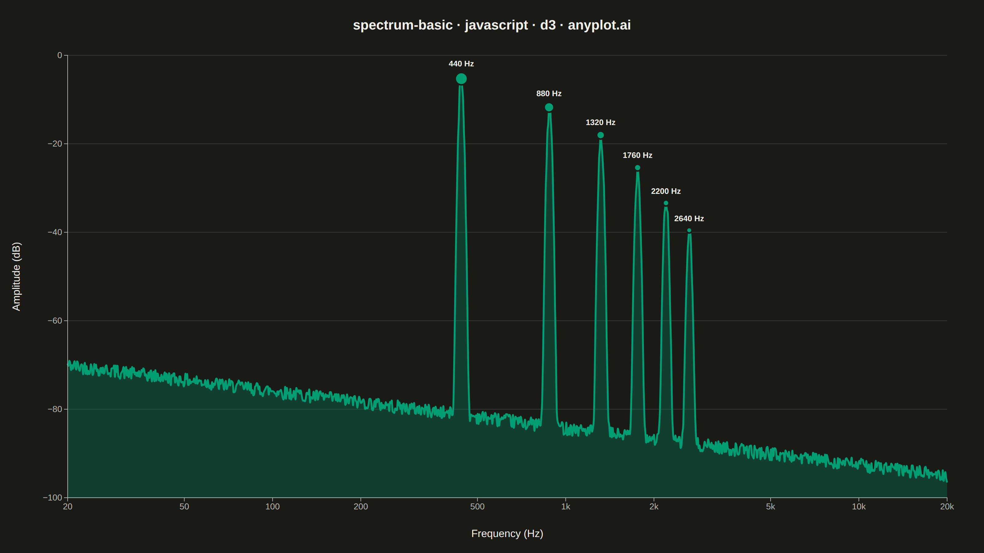
A frequency spectrum plot displays signal amplitude or power across a range of frequencies, showing the frequency domain representation of time-series data. This visualization reveals the frequency components present in a signal, making it essential for identifying dominant frequencies, harmonics, and noise characteristics. It is fundamental in signal processing, audio engineering, and vibration analysis.
// anyplot.ai
// spectrum-basic: Frequency Spectrum Plot
// Library: d3 7.9.0 | JavaScript 22.23.2
// Quality: 94/100 | Created: 2026-09-09

const t = window.ANYPLOT_TOKENS;
const { width, height } = window.ANYPLOT_SIZE;
const margin = { top: 90, right: 60, bottom: 90, left: 110 };
const iw = width - margin.left - margin.right;
const ih = height - margin.top - margin.bottom;

// --- Data (in-memory, deterministic) ----------------------------------------
// Synthetic audio spectrum: a 440 Hz fundamental (A4) with decaying harmonics
// riding on a pink-noise-shaped floor, spanning the audible range 20 Hz-20 kHz.
function mulberry32(seed) {
  let a = seed;
  return function () {
    a |= 0;
    a = (a + 0x6d2b79f5) | 0;
    let x = Math.imul(a ^ (a >>> 15), 1 | a);
    x = (x + Math.imul(x ^ (x >>> 7), 61 | x)) ^ x;
    return ((x ^ (x >>> 14)) >>> 0) / 4294967296;
  };
}
const rand = mulberry32(42);

const FUNDAMENTAL = 440;
const harmonics = d3.range(1, 7).map((n) => ({
  freq: FUNDAMENTAL * n,
  db: -5 - 7 * (n - 1),
  widthOct: 0.02,
}));

const N = 1024;
const fMin = 20;
const fMax = 20000;
const spectrum = d3.range(N).map((i) => {
  const freq = fMin * Math.pow(fMax / fMin, i / (N - 1));

  // Pink-noise-shaped floor: -70 dB at 20 Hz sloping to -95 dB at 20 kHz.
  const octaveFrac =
    (Math.log10(freq) - Math.log10(fMin)) /
    (Math.log10(fMax) - Math.log10(fMin));
  const floorDb = -70 - 25 * octaveFrac;
  let linear = Math.pow(10, floorDb / 20);

  for (const h of harmonics) {
    const distOct = Math.log2(freq / h.freq);
    linear +=
      Math.pow(10, h.db / 20) *
      Math.exp(-0.5 * Math.pow(distOct / h.widthOct, 2));
  }

  const ripple = 1 + (rand() - 0.5) * 0.35;
  linear *= ripple;

  return { freq, db: 20 * Math.log10(linear) };
});

const peaks = harmonics.map((h) => {
  const nearest = spectrum.reduce((best, d) =>
    Math.abs(Math.log2(d.freq / h.freq)) <
    Math.abs(Math.log2(best.freq / h.freq))
      ? d
      : best,
  );
  return nearest;
});

// Peak markers scale with harmonic prominence (linear amplitude, not dB) via a
// sqrt scale, so marker *area* — not radius — tracks acoustic power. The
// fundamental reads as the visually dominant peak; higher harmonics taper off.
const peakAmpLinear = harmonics.map((h) => Math.pow(10, h.db / 20));
const rScale = d3
  .scaleSqrt()
  .domain(d3.extent(peakAmpLinear))
  .range([4.5, 10]);

// --- SVG mount ----------------------------------------------------------------
const svg = d3
  .select("#container")
  .append("svg")
  .attr("width", width)
  .attr("height", height);
const g = svg
  .append("g")
  .attr("transform", `translate(${margin.left},${margin.top})`);

// --- Scales ---------------------------------------------------------------
const x = d3.scaleLog().base(10).domain([fMin, fMax]).range([0, iw]);
const yMin = -100;
const yMax = 0;
const y = d3.scaleLinear().domain([yMin, yMax]).range([ih, 0]);

// --- Gridlines (y-axis only, subtle) ---------------------------------------
g.append("g")
  .selectAll("line")
  .data(y.ticks(6))
  .join("line")
  .attr("x1", 0)
  .attr("x2", iw)
  .attr("y1", (d) => y(d))
  .attr("y2", (d) => y(d))
  .attr("stroke", t.grid)
  .attr("stroke-width", 1);

// --- Area + line -------------------------------------------------------------
const area = d3
  .area()
  .x((d) => x(d.freq))
  .y0(y(yMin))
  .y1((d) => y(d.db))
  .curve(d3.curveMonotoneX);

const line = d3
  .line()
  .x((d) => x(d.freq))
  .y((d) => y(d.db))
  .curve(d3.curveMonotoneX);

g.append("path")
  .datum(spectrum)
  .attr("d", area)
  .attr("fill", t.palette[0])
  .attr("fill-opacity", 0.28);

g.append("path")
  .datum(spectrum)
  .attr("d", line)
  .attr("fill", "none")
  .attr("stroke", t.palette[0])
  .attr("stroke-width", 3);

// --- Harmonic peak markers --------------------------------------------------
g.selectAll("circle")
  .data(peaks)
  .join("circle")
  .attr("cx", (d) => x(d.freq))
  .attr("cy", (d) => y(d.db))
  .attr("r", (d, i) => rScale(peakAmpLinear[i]))
  .attr("fill", t.palette[0])
  .attr("stroke", t.pageBg)
  .attr("stroke-width", 2.5);

// --- Harmonic peak labels ----------------------------------------------------
// Direct numeric labels ("440 Hz") on each harmonic, positioned above its
// marker and then corrected with getBBox — real measured layout from the
// browser's text engine, not an estimate — so labels never clip the plot
// edges or collide with a neighbor even as marker radius/label width vary.
const peakLabels = g
  .selectAll(".peak-label")
  .data(peaks)
  .join("text")
  .attr("class", "peak-label")
  .attr("x", (d) => x(d.freq))
  .attr("y", (d, i) => y(d.db) - rScale(peakAmpLinear[i]) - 10)
  .attr("text-anchor", "middle")
  .attr("fill", t.ink)
  .style("font-size", "13px")
  .style("font-weight", "600")
  .text((d, i) => `${harmonics[i].freq} Hz`);

const labelNodes = peakLabels.nodes();
labelNodes.forEach((node) => {
  const bbox = node.getBBox();
  if (bbox.x < 0) d3.select(node).attr("text-anchor", "start").attr("x", 0);
  else if (bbox.x + bbox.width > iw)
    d3.select(node).attr("text-anchor", "end").attr("x", iw);
});
for (let i = 1; i < labelNodes.length; i++) {
  const prev = labelNodes[i - 1].getBBox();
  const cur = labelNodes[i].getBBox();
  const overlapsX = cur.x < prev.x + prev.width && cur.x + cur.width > prev.x;
  const overlapsY = Math.abs(cur.y - prev.y) < prev.height + 4;
  if (overlapsX && overlapsY) {
    const sel = d3.select(labelNodes[i]);
    sel.attr("y", parseFloat(sel.attr("y")) - (prev.height + 4));
  }
}

// --- Axes --------------------------------------------------------------------
const xTickValues = [20, 50, 100, 200, 500, 1000, 2000, 5000, 10000, 20000];
const xAxis = g
  .append("g")
  .attr("transform", `translate(0,${ih})`)
  .call(
    d3
      .axisBottom(x)
      .tickValues(xTickValues)
      .tickFormat((d) => (d >= 1000 ? `${d / 1000}k` : `${d}`)),
  );

const yAxis = g
  .append("g")
  .call(d3.axisLeft(y).tickValues(d3.range(yMin, yMax + 1, 20)));

for (const ax of [xAxis, yAxis]) {
  ax.selectAll("text").attr("fill", t.inkSoft).style("font-size", "14px");
  ax.selectAll("line").attr("stroke", t.inkSoft);
  ax.select(".domain").attr("stroke", t.inkSoft);
}

// --- Axis labels ---------------------------------------------------------------
g.append("text")
  .attr("x", iw / 2)
  .attr("y", ih + 64)
  .attr("text-anchor", "middle")
  .attr("fill", t.ink)
  .style("font-size", "17px")
  .text("Frequency (Hz)");

g.append("text")
  .attr("transform", `translate(${-78},${ih / 2}) rotate(-90)`)
  .attr("text-anchor", "middle")
  .attr("fill", t.ink)
  .style("font-size", "17px")
  .text("Amplitude (dB)");

// --- Title ---------------------------------------------------------------------
svg
  .append("text")
  .attr("x", width / 2)
  .attr("y", 48)
  .attr("text-anchor", "middle")
  .attr("fill", t.ink)
  .style("font-size", "22px")
  .style("font-weight", "600")
  .text("spectrum-basic · javascript · d3 · anyplot.ai");
Runnable source as JSON, for any HTTP client: https://api.anyplot.ai/specs/spectrum-basic/d3/code. Any spec id and library id listed in llms-full.txt fit the same URL shape; every URL below is complete and callable.
{
  "spec_id": "spectrum-basic",
  "language": "javascript",
  "library": "d3",
  "page": "https://anyplot.ai/spectrum-basic/javascript/d3",
  "hub": "https://anyplot.ai/spectrum-basic",
  "code_json": "https://api.anyplot.ai/specs/spectrum-basic/d3/code",
  "spec_json": "https://api.anyplot.ai/specs/spectrum-basic",
  "render_light_png": "https://storage.googleapis.com/anyplot-images/plots/spectrum-basic/javascript/d3/plot-light.png",
  "render_dark_png": "https://storage.googleapis.com/anyplot-images/plots/spectrum-basic/javascript/d3/plot-dark.png",
  "interactive_light_html": "https://storage.googleapis.com/anyplot-images/plots/spectrum-basic/javascript/d3/plot-light.html",
  "interactive_dark_html": "https://storage.googleapis.com/anyplot-images/plots/spectrum-basic/javascript/d3/plot-dark.html",
  "quality_score": 94.0,
  "license": "MIT",
  "guide": "https://anyplot.ai/llms.txt"
}
Part of Frequency Spectrum Plot on anyplot.ai.