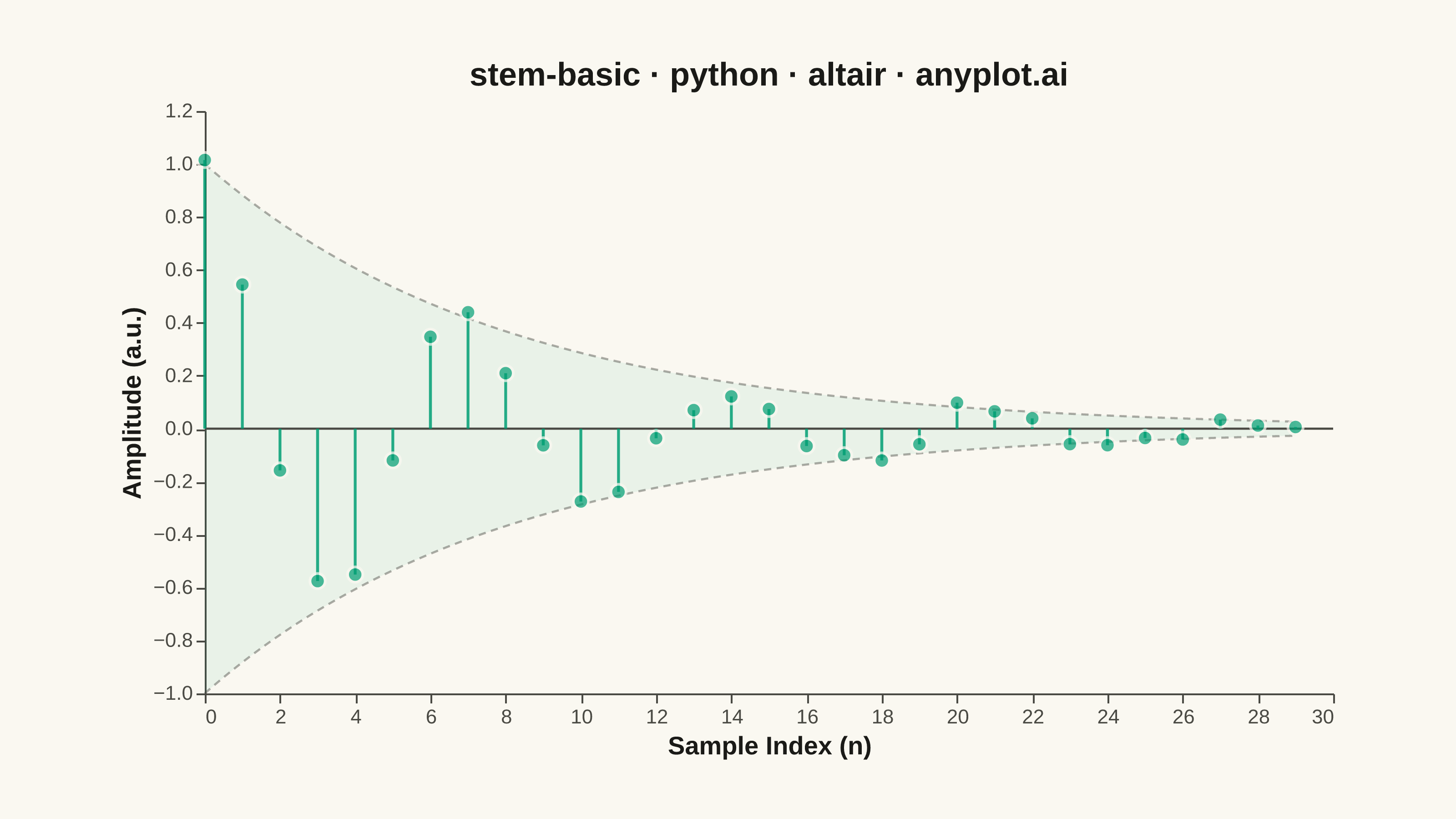
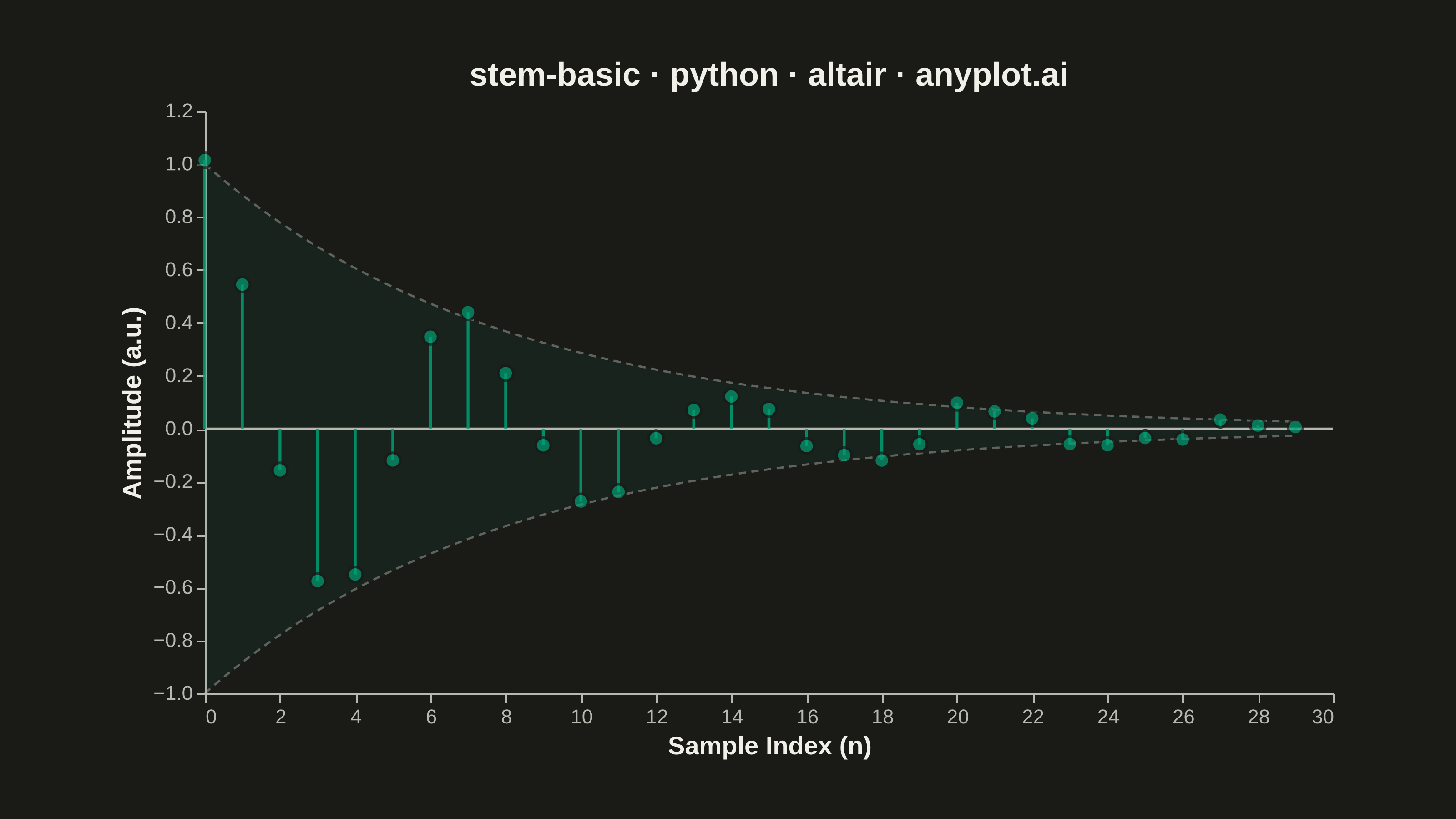
A stem plot displays data points as markers connected to a baseline by vertical lines (stems). Each data point is represented by a marker at the data value with a thin line extending down to a baseline, making it ideal for visualizing discrete or sequential data where individual values matter. This plot type is particularly useful in signal processing and scientific applications where the discrete nature of measurements needs emphasis.
""" anyplot.ai
stem-basic: Basic Stem Plot
Library: altair 6.2.2 | Python 3.13.14
Quality: 91/100 | Updated: 2026-07-25
"""

import os

import altair as alt
import numpy as np
import pandas as pd
from PIL import Image


# Theme tokens
THEME = os.getenv("ANYPLOT_THEME", "light")
PAGE_BG = "#FAF8F1" if THEME == "light" else "#1A1A17"
INK = "#1A1A17" if THEME == "light" else "#F0EFE8"
INK_SOFT = "#4A4A44" if THEME == "light" else "#B8B7B0"
BRAND = "#009E73"  # Imprint palette position 1

# Data — acoustic impulse response samples
np.random.seed(42)
n_samples = 30
sample_index = np.arange(n_samples)
amplitude = np.exp(-sample_index / 8) * np.cos(sample_index * 0.9) + np.random.randn(n_samples) * 0.03

df = pd.DataFrame({"n": sample_index, "amplitude": amplitude, "baseline": 0.0})

# Decay envelope — highlights the exponential decay story
n_env = np.linspace(0, n_samples - 1, 200)
env_df = pd.DataFrame({"n": n_env, "upper": np.exp(-n_env / 8), "lower": -np.exp(-n_env / 8)})

# Shaded decay region (subtle background emphasis)
envelope_area = (
    alt.Chart(env_df)
    .mark_area(color=BRAND, opacity=0.07)
    .encode(x=alt.X("n:Q"), y=alt.Y("upper:Q"), y2=alt.Y2("lower:Q"))
)

# Dashed bounds of the decay envelope
envelope_upper = (
    alt.Chart(env_df)
    .mark_line(color=INK_SOFT, strokeWidth=1.2, strokeDash=[4, 3], opacity=0.45)
    .encode(x=alt.X("n:Q"), y=alt.Y("upper:Q"))
)

envelope_lower = (
    alt.Chart(env_df)
    .mark_line(color=INK_SOFT, strokeWidth=1.2, strokeDash=[4, 3], opacity=0.45)
    .encode(x=alt.X("n:Q"), y=alt.Y("lower:Q"))
)

# Baseline rule at y=0
baseline_rule = alt.Chart(pd.DataFrame({"y": [0]})).mark_rule(color=INK_SOFT, strokeWidth=1.2).encode(y=alt.Y("y:Q"))

# Stems: vertical rules from baseline to each data point
stems = (
    alt.Chart(df)
    .mark_rule(color=BRAND, strokeWidth=1.6, opacity=0.85)
    .encode(
        x=alt.X("n:Q", title="Sample Index (n)", axis=alt.Axis(labelFontSize=11, titleFontSize=14)),
        y=alt.Y("baseline:Q"),
        y2=alt.Y2("amplitude:Q"),
    )
)

# Hover selection — nearest-point highlight, an Altair-distinctive interactive param
# that has no static-PNG equivalent (default state == static render, unaffected).
hover = alt.selection_point(fields=["n"], on="pointerover", nearest=True, empty=False)

# Markers at the tip of each stem
markers = (
    alt.Chart(df)
    .mark_circle(color=BRAND, stroke=PAGE_BG, strokeWidth=1.5)
    .encode(
        x=alt.X("n:Q"),
        y=alt.Y("amplitude:Q", title="Amplitude (a.u.)", axis=alt.Axis(labelFontSize=11, titleFontSize=14)),
        size=alt.condition(hover, alt.value(160), alt.value(70)),
        tooltip=[
            alt.Tooltip("n:Q", title="Sample (n)"),
            alt.Tooltip("amplitude:Q", title="Amplitude (a.u.)", format=".3f"),
        ],
    )
    .add_params(hover)
)

# Compose and apply theme-adaptive chrome
chart = (
    (envelope_area + envelope_upper + envelope_lower + baseline_rule + stems + markers)
    .properties(
        width=620,
        height=320,
        background=PAGE_BG,
        title=alt.Title(
            "stem-basic · python · altair · anyplot.ai", fontSize=18, fontWeight="bold", anchor="middle", color=INK
        ),
    )
    .configure_view(fill=PAGE_BG, stroke=None)
    .configure_axis(
        domainColor=INK_SOFT,
        tickColor=INK_SOFT,
        grid=False,
        labelColor=INK_SOFT,
        titleColor=INK,
        labelFontSize=11,
        titleFontSize=14,
    )
    .configure_title(color=INK, fontSize=18, fontWeight="bold")
)

# Save — hard target: 3200 x 1800 (landscape). See prompts/library/altair.md "Canvas".
chart.save(f"plot-{THEME}.png", scale_factor=4.0)

TW, TH = 3200, 1800
_img = Image.open(f"plot-{THEME}.png").convert("RGB")
_w, _h = _img.size
if _w > TW or _h > TH:
    raise SystemExit(
        f"altair vl-convert produced {_w}x{_h}, exceeds target {TW}x{TH}. "
        f"Shrink chart .properties(width=, height=) values and re-render."
    )
if _w < TW or _h < TH:
    _canvas = Image.new("RGB", (TW, TH), PAGE_BG)
    _canvas.paste(_img, ((TW - _w) // 2, (TH - _h) // 2))
    _canvas.save(f"plot-{THEME}.png")

chart.save(f"plot-{THEME}.html")
Runnable source as JSON, for any HTTP client: https://api.anyplot.ai/specs/stem-basic/altair/code. Any spec id and library id listed in llms-full.txt fit the same URL shape; every URL below is complete and callable.
{
  "spec_id": "stem-basic",
  "language": "python",
  "library": "altair",
  "page": "https://anyplot.ai/stem-basic/python/altair",
  "hub": "https://anyplot.ai/stem-basic",
  "code_json": "https://api.anyplot.ai/specs/stem-basic/altair/code",
  "spec_json": "https://api.anyplot.ai/specs/stem-basic",
  "render_light_png": "https://storage.googleapis.com/anyplot-images/plots/stem-basic/python/altair/plot-light.png",
  "render_dark_png": "https://storage.googleapis.com/anyplot-images/plots/stem-basic/python/altair/plot-dark.png",
  "interactive_light_html": "https://storage.googleapis.com/anyplot-images/plots/stem-basic/python/altair/plot-light.html",
  "interactive_dark_html": "https://storage.googleapis.com/anyplot-images/plots/stem-basic/python/altair/plot-dark.html",
  "quality_score": 91.0,
  "license": "MIT",
  "guide": "https://anyplot.ai/llms.txt"
}
Part of Basic Stem Plot on anyplot.ai.