The same plot in 14 other libraries — JavaScript: Chart.js, D3.js, Apache ECharts, Highcharts; Python: Altair, Bokeh, lets-plot, Matplotlib, Plotly, plotnine, Pygal, Seaborn; R: ggplot2; Julia: Makie.jl. Compare all 15 side by side: Basic Streamline Plot in Python, R, Julia and JavaScript.
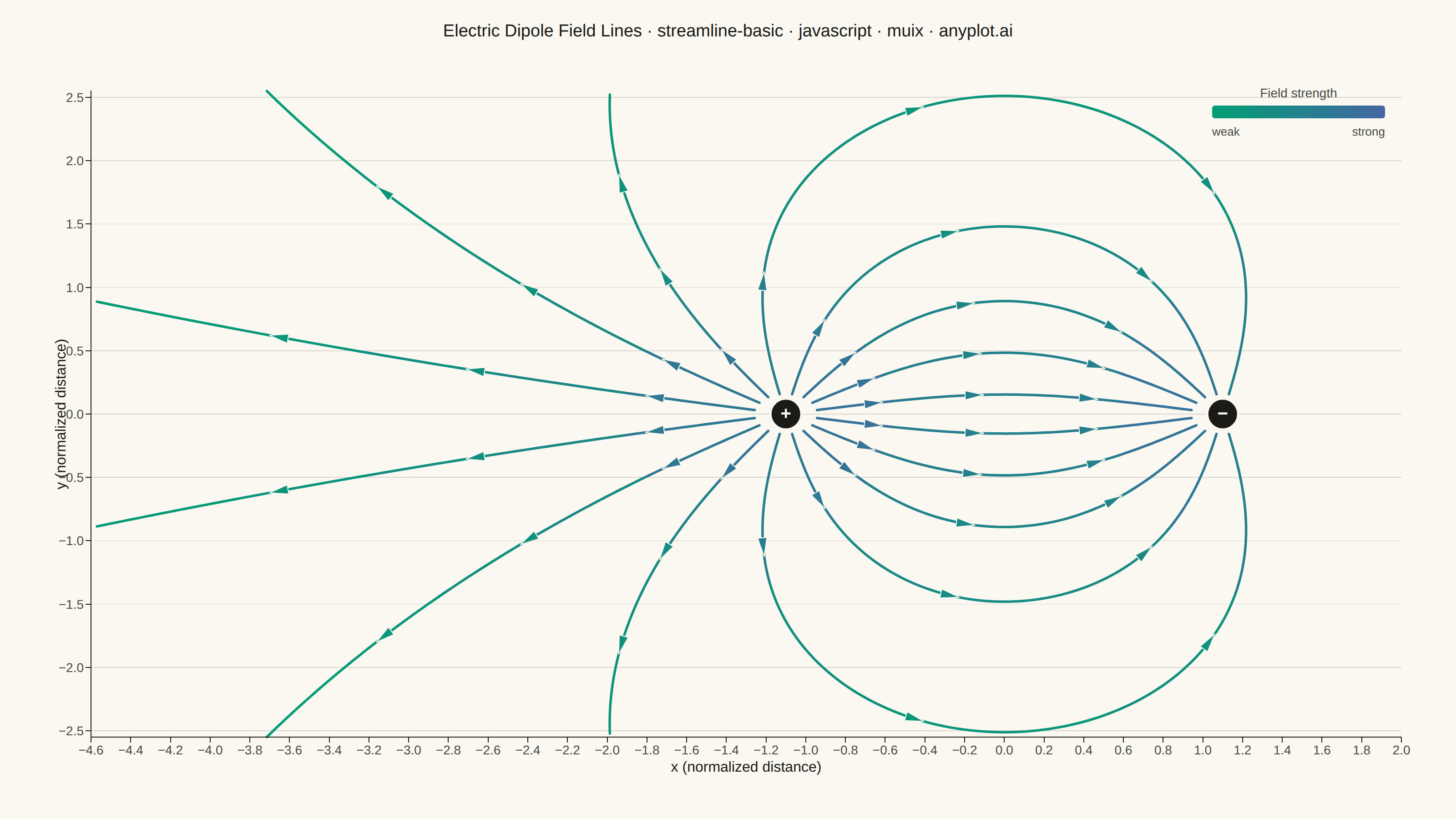
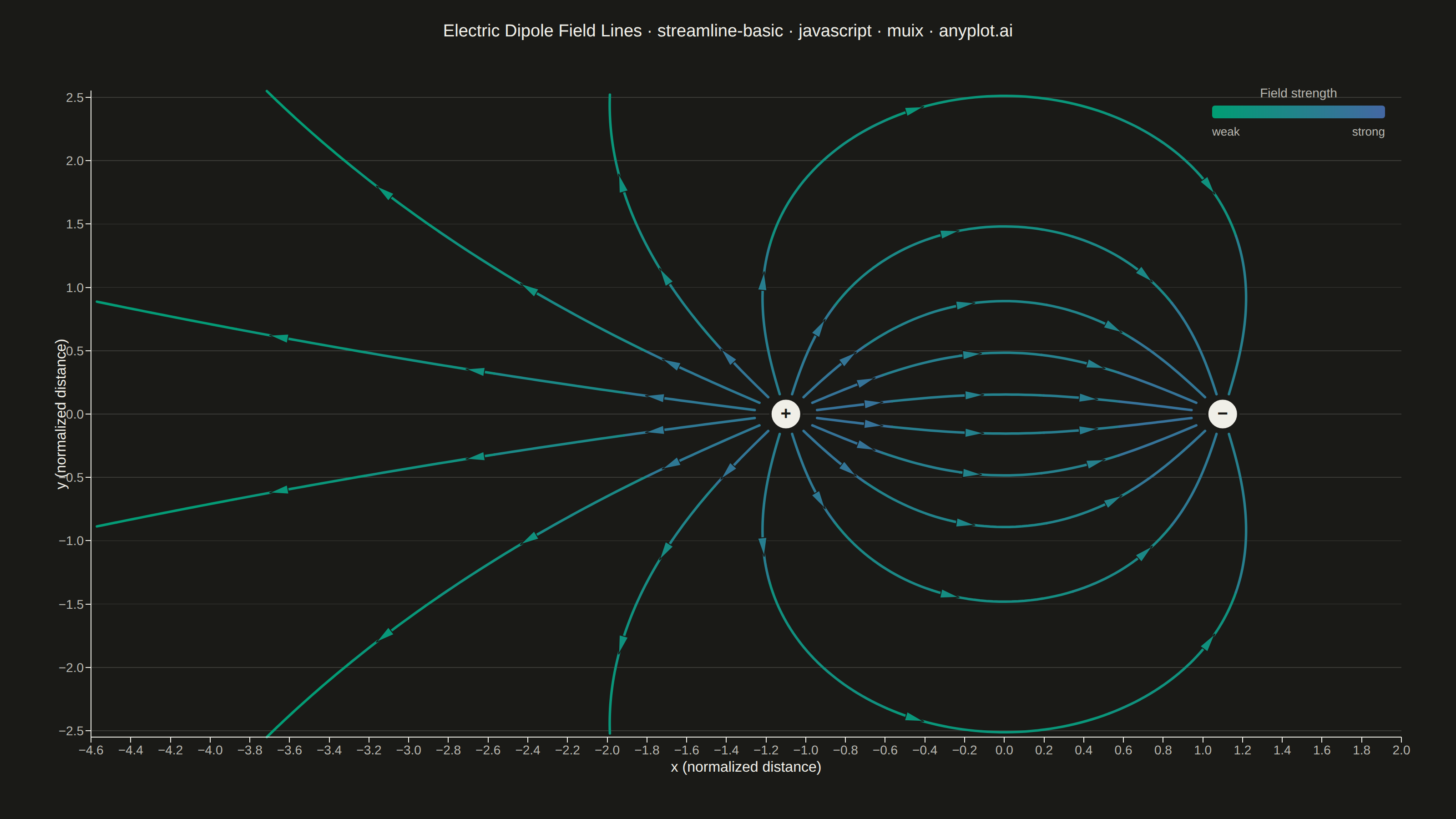
A streamline plot visualizes vector fields using smooth curves that are tangent to the field at every point. Unlike quiver plots that show discrete arrows, streamlines trace continuous paths through the field, revealing flow patterns, circulation, and field topology. This visualization is ideal for understanding fluid dynamics, electromagnetic fields, or gradient fields where the continuous nature of the flow is important.
// anyplot.ai
// streamline-basic: Basic Streamline Plot
// Library: muix 7.29.1 | JavaScript 22.23.2
// Quality: 89/100 | Created: 2026-09-09
import { ChartContainer } from "@mui/x-charts/ChartContainer";
import { LinePlot } from "@mui/x-charts/LineChart";
import { ChartsXAxis } from "@mui/x-charts/ChartsXAxis";
import { ChartsYAxis } from "@mui/x-charts/ChartsYAxis";
import { ChartsGrid } from "@mui/x-charts/ChartsGrid";
import { ChartsText } from "@mui/x-charts/ChartsText";
import { useXScale, useYScale, useDrawingArea } from "@mui/x-charts/hooks";

const t = window.ANYPLOT_TOKENS;

// --- Electric dipole field: two opposite point charges. Field lines are
// traced by RK4 arc-length integration of the *unit* field direction (not a
// closed-form solution) — the canonical "electric/magnetic field line"
// application called out in the spec. u = Ex/|E|, v = Ey/|E|. -------------
const CHARGE_POS = { x: -1.1, y: 0, q: 1 };
const CHARGE_NEG = { x: 1.1, y: 0, q: -1 };
const EXCLUSION_R = 0.16; // seed/terminate radius around each charge (avoids the 1/r^2 singularity)

function fieldAt(x, y) {
  const dxP = x - CHARGE_POS.x;
  const dyP = y - CHARGE_POS.y;
  const dxN = x - CHARGE_NEG.x;
  const dyN = y - CHARGE_NEG.y;
  const rP3 = Math.pow(dxP * dxP + dyP * dyP, 1.5) + 1e-6;
  const rN3 = Math.pow(dxN * dxN + dyN * dyN, 1.5) + 1e-6;
  return [
    CHARGE_POS.q * (dxP / rP3) + CHARGE_NEG.q * (dxN / rN3),
    CHARGE_POS.q * (dyP / rP3) + CHARGE_NEG.q * (dyN / rN3),
  ];
}

function fieldStep(x, y, h) {
  const dir = (px, py) => {
    const [ex, ey] = fieldAt(px, py);
    const mag = Math.hypot(ex, ey) || 1e-9;
    return [ex / mag, ey / mag];
  };
  const [k1x, k1y] = dir(x, y);
  const [k2x, k2y] = dir(x + (h / 2) * k1x, y + (h / 2) * k1y);
  const [k3x, k3y] = dir(x + (h / 2) * k2x, y + (h / 2) * k2y);
  const [k4x, k4y] = dir(x + h * k3x, y + h * k3y);
  return [
    x + (h / 6) * (k1x + 2 * k2x + 2 * k3x + k4x),
    y + (h / 6) * (k1y + 2 * k2y + 2 * k3y + k4y),
  ];
}

const X_BOUND = 4.6;
const Y_BOUND = 2.55;
const STEP_LEN = 0.032;
const MAX_STEPS = 2200;

function traceFieldLine(theta) {
  let x = CHARGE_POS.x + EXCLUSION_R * Math.cos(theta);
  let y = CHARGE_POS.y + EXCLUSION_R * Math.sin(theta);
  const xs = [x];
  const ys = [y];
  const mags = [Math.hypot(...fieldAt(x, y))];
  for (let i = 0; i < MAX_STEPS; i++) {
    [x, y] = fieldStep(x, y, STEP_LEN);
    const dSink = Math.hypot(x - CHARGE_NEG.x, y - CHARGE_NEG.y);
    if (dSink < EXCLUSION_R) {
      const snap = EXCLUSION_R / dSink;
      x = CHARGE_NEG.x + (x - CHARGE_NEG.x) * snap;
      y = CHARGE_NEG.y + (y - CHARGE_NEG.y) * snap;
      xs.push(x);
      ys.push(y);
      mags.push(Math.hypot(...fieldAt(x, y)));
      break;
    }
    if (Math.abs(x) > X_BOUND || Math.abs(y) > Y_BOUND) break;
    xs.push(x);
    ys.push(y);
    mags.push(Math.hypot(...fieldAt(x, y)));
  }
  return { xs, ys, mags };
}

// 16 seeds evenly spaced around the positive charge, offset by half a step so
// none lands on the +/-x axis (the exact axis line never curves back and
// would otherwise run to the domain edge as a degenerate special case).
const LINE_COUNT = 16;
const rawLines = Array.from({ length: LINE_COUNT }, (_, k) =>
  traceFieldLine(((k + 0.5) / LINE_COUNT) * 2 * Math.PI),
);

// --- Color-by-magnitude: MUI X has no per-vertex line coloring, so each
// field line is chopped into fixed sub-segments (own xAxisId + series) and
// each segment gets one solid color from imprint_seq, driven by its average
// log-magnitude — a discretized stand-in for a continuous "speed" colormap.
const allLogMags = rawLines.flatMap((l) => l.mags.map((m) => Math.log10(m + 1e-6)));
const LOG_MIN = Math.min(...allLogMags);
const LOG_MAX = Math.max(...allLogMags);

function hexToRgb(hex) {
  const n = parseInt(hex.slice(1), 16);
  return [(n >> 16) & 255, (n >> 8) & 255, n & 255];
}
function lerpColor(hexA, hexB, f) {
  const a = hexToRgb(hexA);
  const b = hexToRgb(hexB);
  const c = a.map((v, i) => Math.round(v + (b[i] - v) * Math.min(1, Math.max(0, f))));
  return `rgb(${c[0]}, ${c[1]}, ${c[2]})`;
}

const SEGMENTS_PER_LINE = 5;
let axisCounter = 0;
const segments = [];
const arrowSpecs = [];

for (const line of rawLines) {
  const n = line.xs.length;
  const segLen = Math.max(1, Math.floor((n - 1) / SEGMENTS_PER_LINE));
  const lineSegments = [];
  for (let s = 0; s < SEGMENTS_PER_LINE; s++) {
    const start = s * segLen;
    const end = s === SEGMENTS_PER_LINE - 1 ? n - 1 : (s + 1) * segLen;
    if (end <= start) continue;
    const segMags = line.mags.slice(start, end + 1);
    const avgLogMag = segMags.reduce((acc, m) => acc + Math.log10(m + 1e-6), 0) / segMags.length;
    const norm = LOG_MAX > LOG_MIN ? (avgLogMag - LOG_MIN) / (LOG_MAX - LOG_MIN) : 0.5;
    const segment = {
      axisId: `fl-${axisCounter++}`,
      xs: line.xs.slice(start, end + 1),
      ys: line.ys.slice(start, end + 1),
      color: lerpColor(t.seq[0], t.seq[1], norm),
    };
    segments.push(segment);
    lineSegments.push(segment);
  }
  // Direction arrows at two points along the raw path, colored to match the
  // local field-strength segment they fall in.
  if (n > 12 && lineSegments.length > 0) {
    [0.15, 0.42, 0.72].forEach((frac) => {
      const idx = Math.min(n - 3, Math.max(2, Math.round(frac * (n - 1))));
      const segIdx = Math.min(lineSegments.length - 1, Math.floor(idx / segLen));
      const segment = lineSegments[segIdx];
      arrowSpecs.push({
        x0: line.xs[idx],
        y0: line.ys[idx],
        x1: line.xs[idx + 2],
        y1: line.ys[idx + 2],
        color: segment.color,
      });
    });
  }
}

const SHARED_AXIS_ID = segments[0].axisId; // every xAxis shares the same explicit
// [X_MIN, X_MAX] linear domain, so any one of them maps data->pixels for all lines.

// Display domain is tighter than the integration bound X_BOUND on the right:
// this dipole's field lines either loop between the two charges or escape
// toward -x, so nothing ever occupies the right two-thirds of a symmetric
// domain — cropping it there fills the canvas instead of framing empty space.
const X_MIN = -X_BOUND;
const X_MAX = 2.0;
const Y_MIN = -Y_BOUND;
const Y_MAX = Y_BOUND;

const TITLE = "Electric Dipole Field Lines · streamline-basic · javascript · muix · anyplot.ai";
const TITLE_HEIGHT = 70;
const TITLE_FONT_SIZE = Math.max(15, Math.round(22 * Math.min(1, 67 / TITLE.length)));

const MARGIN = { top: 30, bottom: 90, left: 100, right: 60 };

function arrowPoints(cx, cy, angle, size) {
  const backAngle = angle + Math.PI;
  const spread = 0.48;
  const tip = [cx + Math.cos(angle) * size, cy + Math.sin(angle) * size];
  const left = [cx + Math.cos(backAngle - spread) * size, cy + Math.sin(backAngle - spread) * size];
  const right = [cx + Math.cos(backAngle + spread) * size, cy + Math.sin(backAngle + spread) * size];
  return `${tip.join(",")} ${left.join(",")} ${right.join(",")}`;
}

// --- Custom overlay: charge markers, direction arrowheads, and a manual
// field-strength gradient legend (community x-charts has no bound color-axis
// legend wired for a line chart, so the swatch is drawn directly). ----------
function FieldOverlay() {
  const xScale = useXScale(SHARED_AXIS_ID);
  const yScale = useYScale();
  const area = useDrawingArea();

  const posPx = { x: xScale(CHARGE_POS.x), y: yScale(CHARGE_POS.y) };
  const negPx = { x: xScale(CHARGE_NEG.x), y: yScale(CHARGE_NEG.y) };

  const legendW = 190;
  const legendH = 14;
  const legendX = area.left + area.width - legendW - 18;
  const legendY = area.top + 16;

  return (
    <g>
      {arrowSpecs.map((a, i) => {
        const p0 = { x: xScale(a.x0), y: yScale(a.y0) };
        const p1 = { x: xScale(a.x1), y: yScale(a.y1) };
        const angle = Math.atan2(p1.y - p0.y, p1.x - p0.x);
        return (
          <polygon
            key={i}
            points={arrowPoints(p0.x, p0.y, angle, 11)}
            fill={a.color}
            stroke={t.pageBg}
            strokeWidth={1}
          />
        );
      })}

      <circle cx={posPx.x} cy={posPx.y} r={17} fill={t.ink} stroke={t.pageBg} strokeWidth={2.5} />
      <ChartsText
        x={posPx.x}
        y={posPx.y}
        text="+"
        style={{ fontSize: 20, fontWeight: 700, fill: t.pageBg, textAnchor: "middle", dominantBaseline: "central" }}
      />
      <circle cx={negPx.x} cy={negPx.y} r={17} fill={t.ink} stroke={t.pageBg} strokeWidth={2.5} />
      <ChartsText
        x={negPx.x}
        y={negPx.y}
        text="−"
        style={{ fontSize: 20, fontWeight: 700, fill: t.pageBg, textAnchor: "middle", dominantBaseline: "central" }}
      />

      <defs>
        <linearGradient id="streamline-strength-grad" x1="0" y1="0" x2="1" y2="0">
          <stop offset="0%" stopColor={t.seq[0]} />
          <stop offset="100%" stopColor={t.seq[1]} />
        </linearGradient>
      </defs>
      <ChartsText
        x={legendX + legendW / 2}
        y={legendY - 14}
        text="Field strength"
        style={{ fontSize: 14, fill: t.inkSoft, textAnchor: "middle", dominantBaseline: "central" }}
      />
      <rect x={legendX} y={legendY} width={legendW} height={legendH} rx={3} fill="url(#streamline-strength-grad)" />
      <ChartsText
        x={legendX}
        y={legendY + legendH + 14}
        text="weak"
        style={{ fontSize: 13, fill: t.inkSoft, textAnchor: "start", dominantBaseline: "central" }}
      />
      <ChartsText
        x={legendX + legendW}
        y={legendY + legendH + 14}
        text="strong"
        style={{ fontSize: 13, fill: t.inkSoft, textAnchor: "end", dominantBaseline: "central" }}
      />
    </g>
  );
}

// --- Chart (default-exported component — the harness mounts it) -------------
export default function Chart() {
  return (
    <div
      style={{
        width: window.ANYPLOT_SIZE.width,
        height: window.ANYPLOT_SIZE.height,
        display: "flex",
        flexDirection: "column",
      }}
    >
      <div
        style={{
          height: TITLE_HEIGHT,
          display: "flex",
          alignItems: "center",
          justifyContent: "center",
          fontSize: TITLE_FONT_SIZE,
          fontWeight: 500,
          color: t.ink,
        }}
      >
        {TITLE}
      </div>
      <ChartContainer
        width={window.ANYPLOT_SIZE.width}
        height={window.ANYPLOT_SIZE.height - TITLE_HEIGHT}
        margin={MARGIN}
        skipAnimation
        sx={{
          ".MuiLineElement-root": { strokeWidth: 2.75, strokeLinecap: "round" },
          "& .MuiChartsGrid-line": { stroke: t.grid, strokeWidth: 0.75 },
        }}
        xAxis={segments.map((seg) => ({
          id: seg.axisId,
          scaleType: "linear",
          data: seg.xs,
          min: X_MIN,
          max: X_MAX,
        }))}
        yAxis={[{ scaleType: "linear", min: Y_MIN, max: Y_MAX }]}
        series={segments.map((seg) => ({
          type: "line",
          data: seg.ys,
          xAxisId: seg.axisId,
          color: seg.color,
          curve: "linear",
          showMark: false,
        }))}
      >
        <ChartsGrid horizontal />
        <LinePlot />
        <FieldOverlay />
        <ChartsXAxis
          axisId={SHARED_AXIS_ID}
          label="x (normalized distance)"
          labelStyle={{ fontSize: 16, fill: t.ink, fontWeight: 500 }}
          tickLabelStyle={{ fontSize: 14, fill: t.inkSoft }}
          stroke={t.inkSoft}
        />
        <ChartsYAxis
          label="y (normalized distance)"
          labelStyle={{ fontSize: 16, fill: t.ink, fontWeight: 500 }}
          tickLabelStyle={{ fontSize: 14, fill: t.inkSoft }}
          stroke={t.inkSoft}
        />
      </ChartContainer>
    </div>
  );
}
Runnable source as JSON, for any HTTP client: https://api.anyplot.ai/specs/streamline-basic/muix/code. Any spec id and library id listed in llms-full.txt fit the same URL shape; every URL below is complete and callable.
{
  "spec_id": "streamline-basic",
  "language": "javascript",
  "library": "muix",
  "page": "https://anyplot.ai/streamline-basic/javascript/muix",
  "hub": "https://anyplot.ai/streamline-basic",
  "code_json": "https://api.anyplot.ai/specs/streamline-basic/muix/code",
  "spec_json": "https://api.anyplot.ai/specs/streamline-basic",
  "render_light_png": "https://storage.googleapis.com/anyplot-images/plots/streamline-basic/javascript/muix/plot-light.png",
  "render_dark_png": "https://storage.googleapis.com/anyplot-images/plots/streamline-basic/javascript/muix/plot-dark.png",
  "interactive_light_html": "https://storage.googleapis.com/anyplot-images/plots/streamline-basic/javascript/muix/plot-light.html",
  "interactive_dark_html": "https://storage.googleapis.com/anyplot-images/plots/streamline-basic/javascript/muix/plot-dark.html",
  "quality_score": 89.0,
  "license": "MIT",
  "guide": "https://anyplot.ai/llms.txt"
}
Part of Basic Streamline Plot on anyplot.ai.