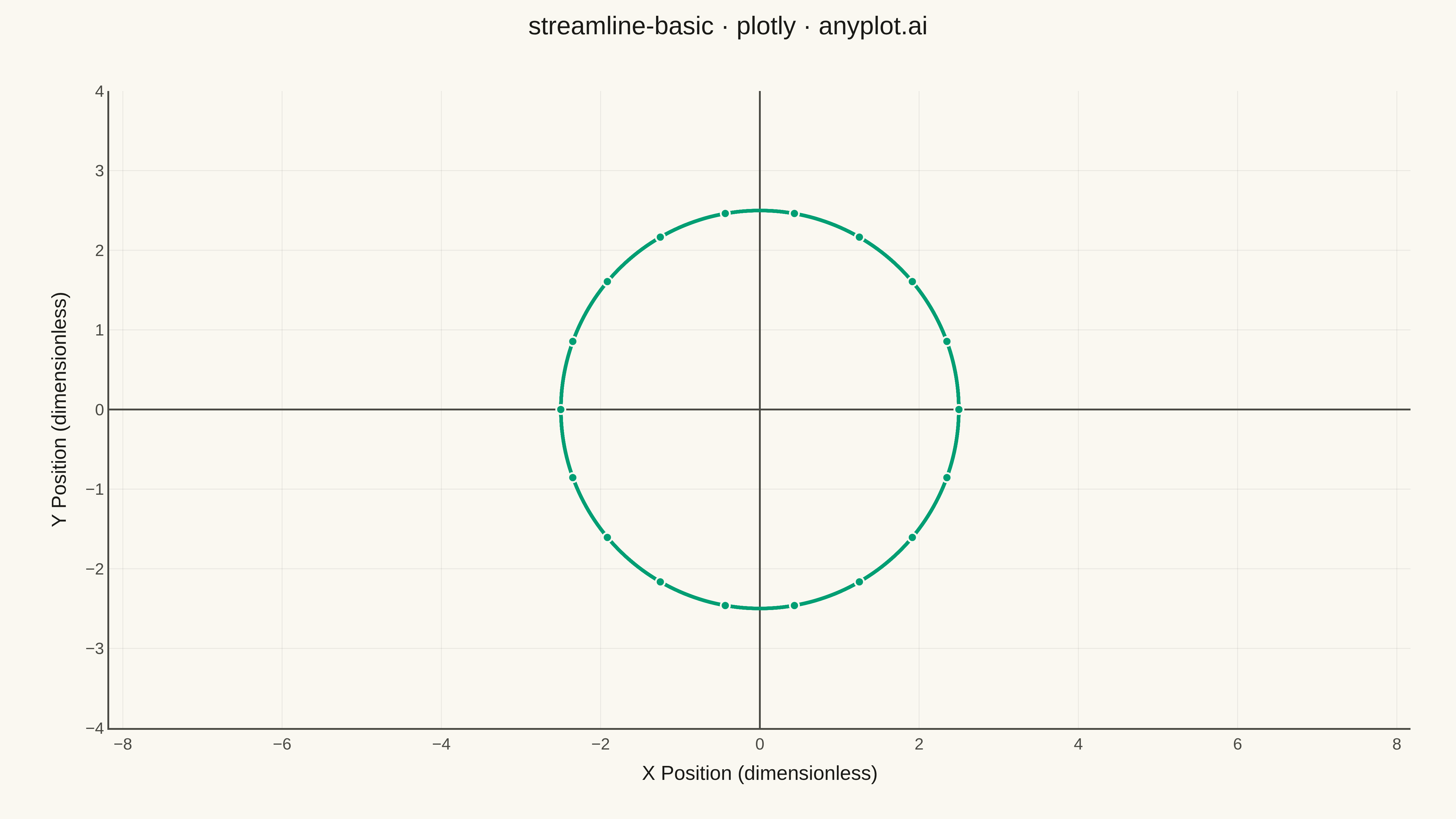
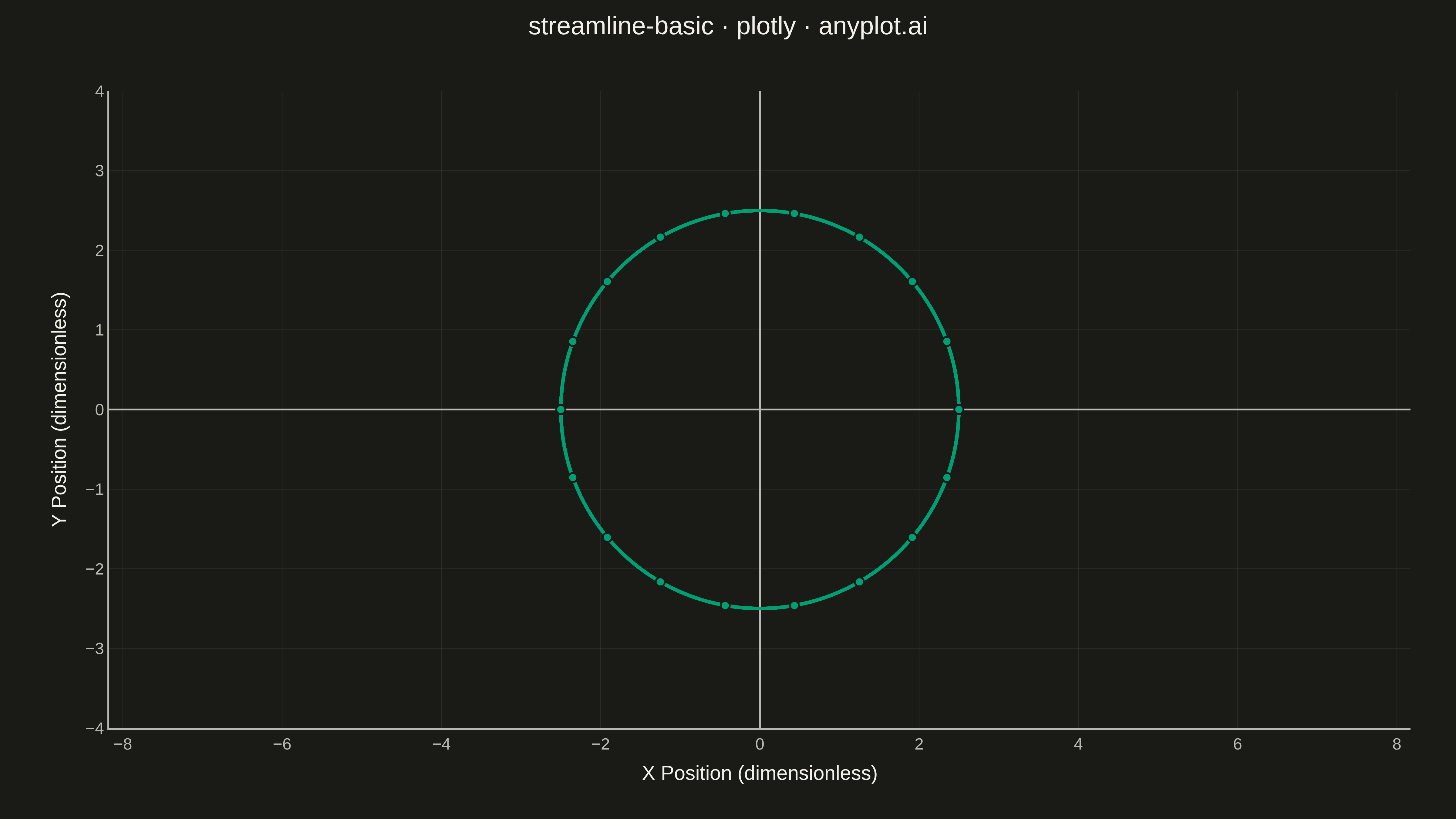
A streamline plot visualizes vector fields using smooth curves that are tangent to the field at every point. Unlike quiver plots that show discrete arrows, streamlines trace continuous paths through the field, revealing flow patterns, circulation, and field topology. This visualization is ideal for understanding fluid dynamics, electromagnetic fields, or gradient fields where the continuous nature of the flow is important.
""" anyplot.ai
streamline-basic: Basic Streamline Plot
Library: plotly 6.7.0 | Python 3.13.13
Quality: 91/100 | Updated: 2026-05-14
"""

import os

import numpy as np
import plotly.graph_objects as go
from scipy.integrate import solve_ivp


# Theme tokens
THEME = os.getenv("ANYPLOT_THEME", "light")
PAGE_BG = "#FAF8F1" if THEME == "light" else "#1A1A17"
INK = "#1A1A17" if THEME == "light" else "#F0EFE8"
INK_SOFT = "#4A4A44" if THEME == "light" else "#B8B7B0"
GRID = "rgba(26,26,23,0.10)" if THEME == "light" else "rgba(240,239,232,0.10)"
BRAND = "#009E73"

# Data - Vortex flow field: u = -y, v = x (circular streamlines)
fig = go.Figure()


# Function to compute velocity at any point
def velocity_field(t, state):
    x, y = state
    dx = -y
    dy = x
    return [dx, dy]


# Create streamlines from starting points on a circle
num_streamlines = 18
for angle in np.linspace(0, 2 * np.pi, num_streamlines, endpoint=False):
    start_x = 2.5 * np.cos(angle)
    start_y = 2.5 * np.sin(angle)

    # Integrate forward
    sol_forward = solve_ivp(
        velocity_field, (0, 5), [start_x, start_y], t_eval=np.linspace(0, 5, 150), dense_output=True
    )

    # Integrate backward
    sol_backward = solve_ivp(
        velocity_field, (0, -5), [start_x, start_y], t_eval=np.linspace(0, -5, 150), dense_output=True
    )

    # Plot forward streamline
    if sol_forward.t.size > 0:
        fig.add_trace(
            go.Scatter(
                x=sol_forward.y[0],
                y=sol_forward.y[1],
                mode="lines",
                line={"color": BRAND, "width": 3},
                hoverinfo="none",
                showlegend=False,
            )
        )

    # Plot backward streamline
    if sol_backward.t.size > 0:
        fig.add_trace(
            go.Scatter(
                x=sol_backward.y[0],
                y=sol_backward.y[1],
                mode="lines",
                line={"color": BRAND, "width": 3},
                hoverinfo="none",
                showlegend=False,
            )
        )

# Update layout for large canvas with theme support
fig.update_layout(
    title={"text": "streamline-basic · plotly · anyplot.ai", "font": {"size": 28, "color": INK}, "x": 0.5, "xanchor": "center"},
    xaxis={
        "title": {"text": "X Position (dimensionless)", "font": {"size": 22, "color": INK}},
        "tickfont": {"size": 18, "color": INK_SOFT},
        "showgrid": True,
        "gridwidth": 1,
        "gridcolor": GRID,
        "zeroline": True,
        "zerolinewidth": 2,
        "zerolinecolor": INK_SOFT,
        "range": [-4, 4],
        "autorange": False,
        "linecolor": INK_SOFT,
    },
    yaxis={
        "title": {"text": "Y Position (dimensionless)", "font": {"size": 22, "color": INK}},
        "tickfont": {"size": 18, "color": INK_SOFT},
        "showgrid": True,
        "gridwidth": 1,
        "gridcolor": GRID,
        "zeroline": True,
        "zerolinewidth": 2,
        "zerolinecolor": INK_SOFT,
        "range": [-4, 4],
        "autorange": False,
        "scaleanchor": "x",
        "scaleratio": 1,
        "linecolor": INK_SOFT,
    },
    paper_bgcolor=PAGE_BG,
    plot_bgcolor=PAGE_BG,
    font={"color": INK},
    margin={"l": 120, "r": 50, "t": 100, "b": 100},
    showlegend=False,
)

# Save as PNG and HTML
fig.write_image(f"plot-{THEME}.png", width=1600, height=900, scale=3)
fig.write_html(f"plot-{THEME}.html", include_plotlyjs="cdn")
Runnable source as JSON, for any HTTP client: https://api.anyplot.ai/specs/streamline-basic/plotly/code. Any spec id and library id listed in llms-full.txt fit the same URL shape; every URL below is complete and callable.
{
  "spec_id": "streamline-basic",
  "language": "python",
  "library": "plotly",
  "page": "https://anyplot.ai/streamline-basic/python/plotly",
  "hub": "https://anyplot.ai/streamline-basic",
  "code_json": "https://api.anyplot.ai/specs/streamline-basic/plotly/code",
  "spec_json": "https://api.anyplot.ai/specs/streamline-basic",
  "render_light_png": "https://storage.googleapis.com/anyplot-images/plots/streamline-basic/python/plotly/plot-light.png",
  "render_dark_png": "https://storage.googleapis.com/anyplot-images/plots/streamline-basic/python/plotly/plot-dark.png",
  "interactive_light_html": "https://storage.googleapis.com/anyplot-images/plots/streamline-basic/python/plotly/plot-light.html",
  "interactive_dark_html": "https://storage.googleapis.com/anyplot-images/plots/streamline-basic/python/plotly/plot-dark.html",
  "quality_score": 91.0,
  "license": "MIT",
  "guide": "https://anyplot.ai/llms.txt"
}
Part of Basic Streamline Plot on anyplot.ai.