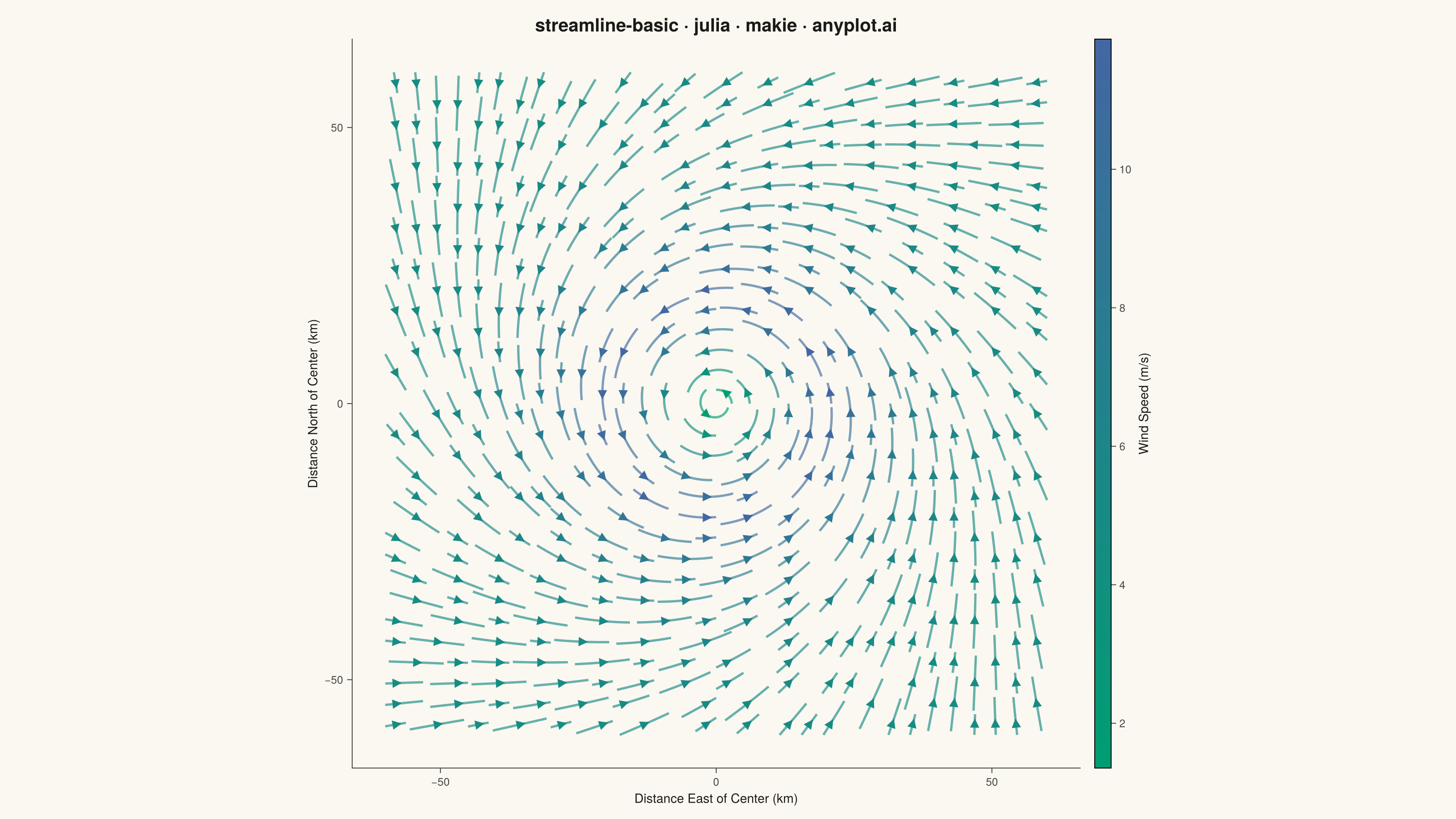
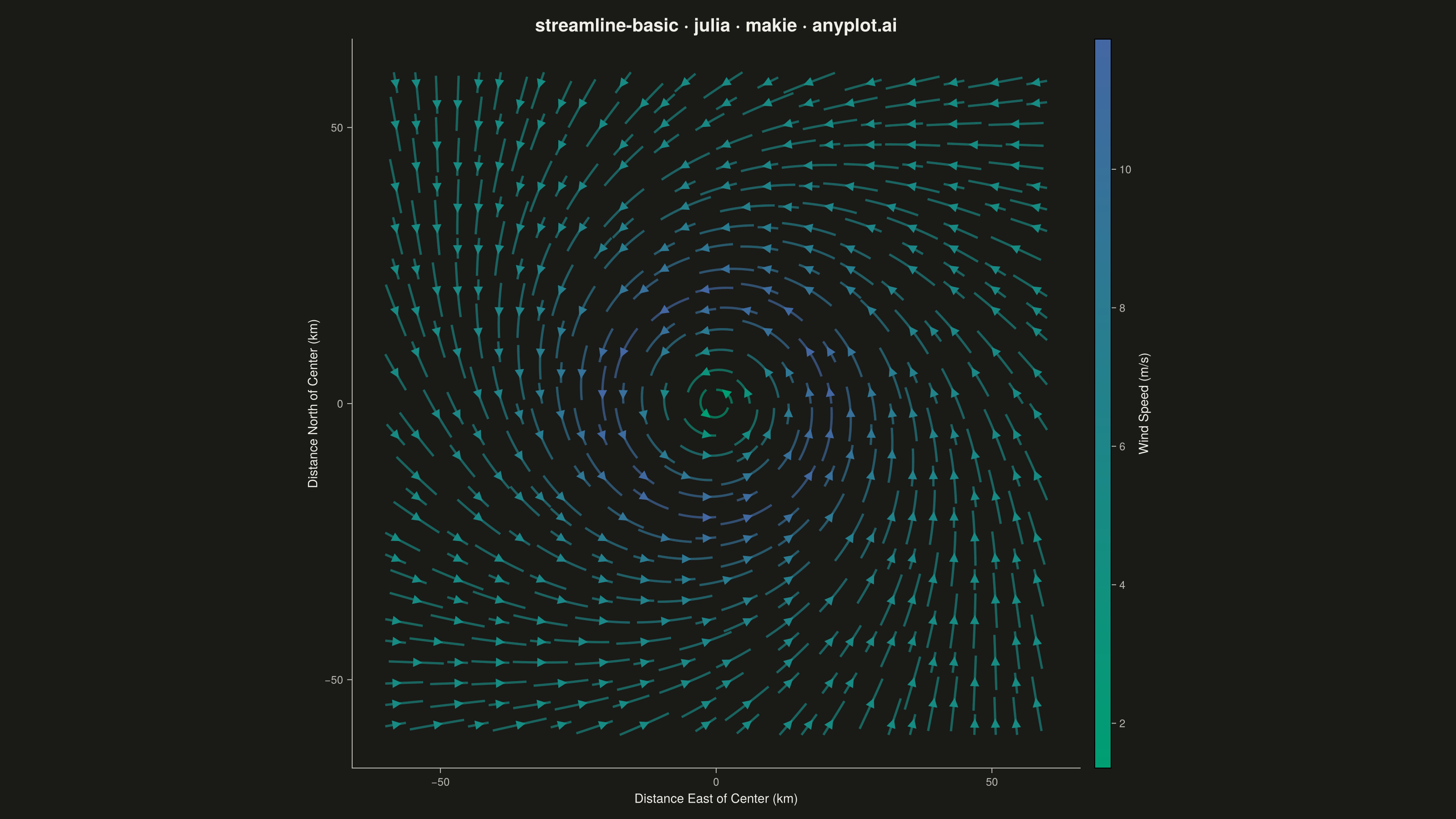
The same plot in 14 other libraries — Python: Altair, Bokeh, lets-plot, Matplotlib, Plotly, plotnine, Pygal, Seaborn; R: ggplot2; JavaScript: Chart.js, D3.js, Apache ECharts, Highcharts, MUI X Charts. Compare all 15 side by side: Basic Streamline Plot in Python, R, Julia and JavaScript.
A streamline plot visualizes vector fields using smooth curves that are tangent to the field at every point. Unlike quiver plots that show discrete arrows, streamlines trace continuous paths through the field, revealing flow patterns, circulation, and field topology. This visualization is ideal for understanding fluid dynamics, electromagnetic fields, or gradient fields where the continuous nature of the flow is important.
# anyplot.ai
# streamline-basic: Basic Streamline Plot
# Library: makie 0.21.9 | Julia 1.11.9
# Quality: 91/100 | Created: 2026-09-09

using CairoMakie
using LinearAlgebra

# --- Theme tokens (see prompts/default-style-guide.md "Theme-adaptive Chrome")
const THEME    = get(ENV, "ANYPLOT_THEME", "light")
const PAGE_BG  = THEME == "light" ? colorant"#FAF8F1" : colorant"#1A1A17"
const INK      = THEME == "light" ? colorant"#1A1A17" : colorant"#F0EFE8"
const INK_SOFT = THEME == "light" ? colorant"#4A4A44" : colorant"#B8B7B0"

# --- Data: wind spiraling into a low-pressure system (Rankine vortex core --
# with a mild radial inflow), the classic cyclone pattern in synoptic charts.
function wind_velocity(x, y)
    r = sqrt(x^2 + y^2) + 1.0e-6
    core_radius = 20.0
    omega = 0.6
    tangential = r <= core_radius ? omega * r : omega * core_radius^2 / r
    inflow = -0.05 * r
    theta = atan(y, x)
    u = -tangential * sin(theta) + inflow * cos(theta)
    v = tangential * cos(theta) + inflow * sin(theta)
    return Point2f(u, v)
end

imprint_seq = cgrad([colorant"#009E73", colorant"#4467A3"])

# --- Plot ---------------------------------------------------------------------
fig = Figure(
    size            = (1600, 900),
    fontsize        = 14,
    backgroundcolor = PAGE_BG,
)

ax = Axis(
    fig[1, 1];
    title             = "streamline-basic · julia · makie · anyplot.ai",
    titlesize         = 20,
    titlecolor        = INK,
    xlabel            = "Distance East of Center (km)",
    ylabel            = "Distance North of Center (km)",
    xlabelsize        = 14,
    ylabelsize        = 14,
    xlabelcolor       = INK,
    ylabelcolor       = INK,
    xticklabelsize    = 12,
    yticklabelsize    = 12,
    xticklabelcolor   = INK_SOFT,
    yticklabelcolor   = INK_SOFT,
    xtickcolor        = INK_SOFT,
    ytickcolor        = INK_SOFT,
    backgroundcolor   = PAGE_BG,
    topspinevisible   = false,
    rightspinevisible = false,
    leftspinecolor    = INK_SOFT,
    bottomspinecolor  = INK_SOFT,
    xgridvisible      = false,
    ygridvisible      = false,
    aspect            = DataAspect(),
)

streamlines = streamplot!(
    ax, wind_velocity, -60.0 .. 60.0, -60.0 .. 60.0;
    color = p -> norm(p),
    colormap = imprint_seq,
    gridsize = (32, 32),
    arrow_size = 14,
    linewidth = 2.5,
)

Colorbar(
    fig[1, 2], streamlines;
    label = "Wind Speed (m/s)",
    labelsize = 14,
    labelcolor = INK,
    ticklabelsize = 12,
    ticklabelcolor = INK_SOFT,
    tickcolor = INK_SOFT,
    width = 18,
)

# DataAspect() forces the axis into a square; tie the column width to the row
# height (rather than a fixed Relative share of the figure) so the colorbar
# hugs the axis instead of floating in leftover 16:9 whitespace.
colsize!(fig.layout, 1, Aspect(1, 1.0))
colgap!(fig.layout, 1, 16)

# --- Save ----------------------------------------------------------------------
save("plot-$(THEME).png", fig; px_per_unit = 2)
Runnable source as JSON, for any HTTP client: https://api.anyplot.ai/specs/streamline-basic/makie/code. Any spec id and library id listed in llms-full.txt fit the same URL shape; every URL below is complete and callable.
{
  "spec_id": "streamline-basic",
  "language": "julia",
  "library": "makie",
  "page": "https://anyplot.ai/streamline-basic/julia/makie",
  "hub": "https://anyplot.ai/streamline-basic",
  "code_json": "https://api.anyplot.ai/specs/streamline-basic/makie/code",
  "spec_json": "https://api.anyplot.ai/specs/streamline-basic",
  "render_light_png": "https://storage.googleapis.com/anyplot-images/plots/streamline-basic/julia/makie/plot-light.png",
  "render_dark_png": "https://storage.googleapis.com/anyplot-images/plots/streamline-basic/julia/makie/plot-dark.png",
  "quality_score": 91.0,
  "license": "MIT",
  "guide": "https://anyplot.ai/llms.txt"
}
Part of Basic Streamline Plot on anyplot.ai.