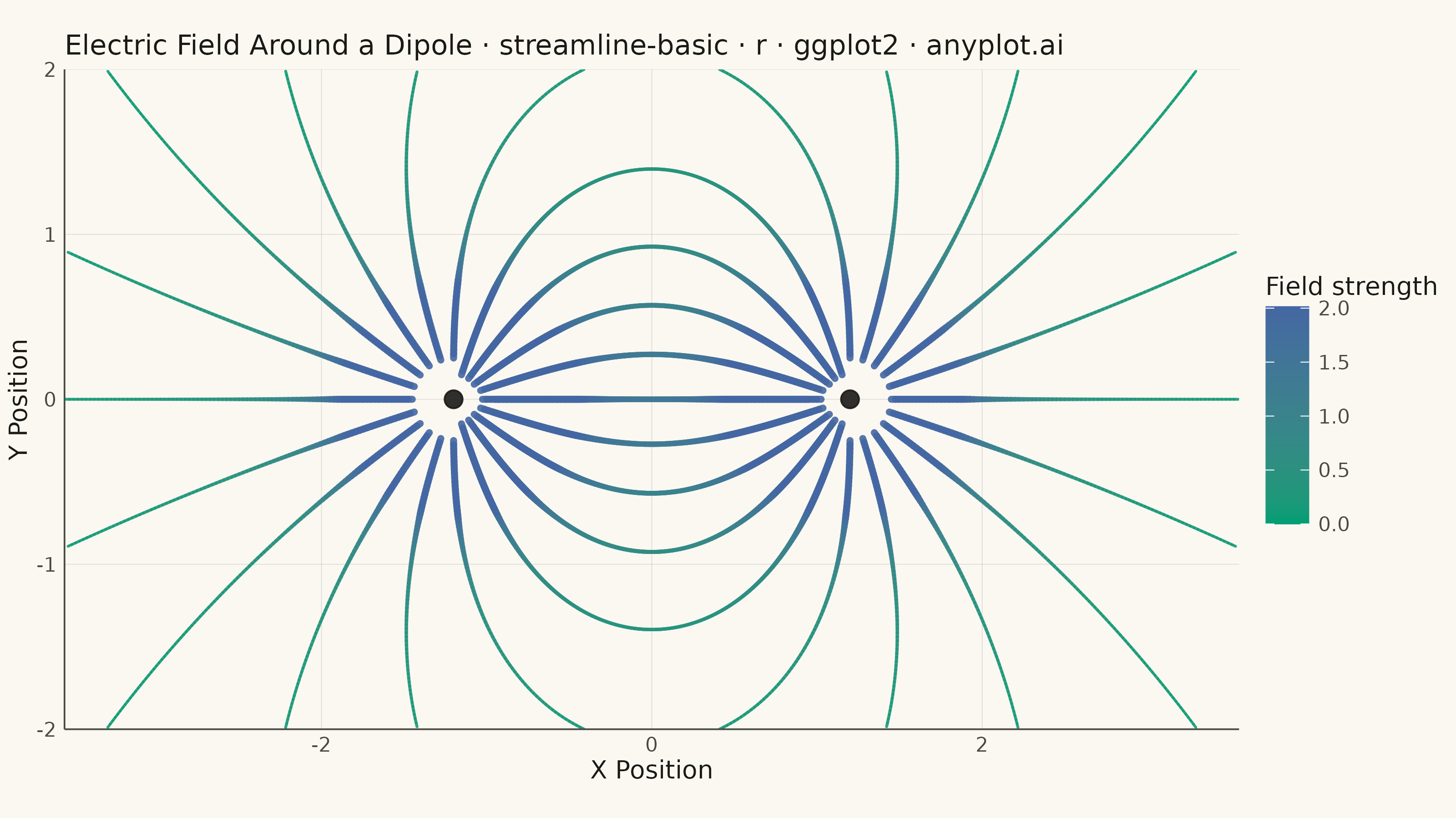
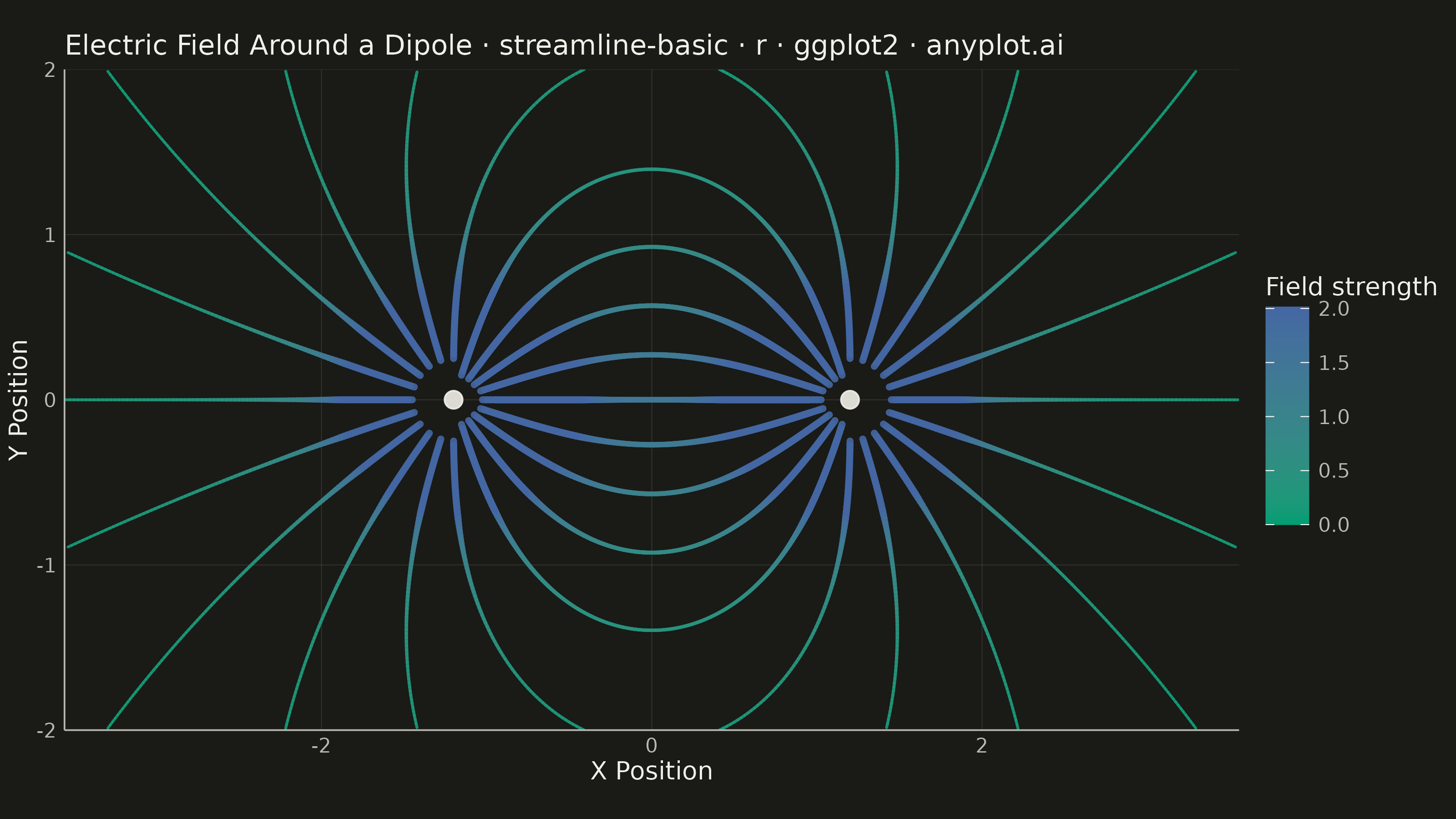
The same plot in 14 other libraries — Python: Altair, Bokeh, lets-plot, Matplotlib, Plotly, plotnine, Pygal, Seaborn; Julia: Makie.jl; JavaScript: Chart.js, D3.js, Apache ECharts, Highcharts, MUI X Charts. Compare all 15 side by side: Basic Streamline Plot in Python, R, Julia and JavaScript.
A streamline plot visualizes vector fields using smooth curves that are tangent to the field at every point. Unlike quiver plots that show discrete arrows, streamlines trace continuous paths through the field, revealing flow patterns, circulation, and field topology. This visualization is ideal for understanding fluid dynamics, electromagnetic fields, or gradient fields where the continuous nature of the flow is important.
#' anyplot.ai
#' streamline-basic: Basic Streamline Plot
#' Library: ggplot2 3.5.1 | R 4.4.1
#' Quality: 92/100 | Created: 2026-09-09

library(ggplot2)
library(dplyr)
library(ragg)

set.seed(42)

# --- Theme tokens -------------------------------------------------------
THEME       <- Sys.getenv("ANYPLOT_THEME", "light")
PAGE_BG     <- if (THEME == "light") "#FAF8F1" else "#1A1A17"
INK         <- if (THEME == "light") "#1A1A17" else "#F0EFE8"
INK_SOFT    <- if (THEME == "light") "#4A4A44" else "#B8B7B0"
IMPRINT_SEQ_LOW  <- "#009E73"  # Imprint sequential cmap, low end
IMPRINT_SEQ_HIGH <- "#4467A3"  # Imprint sequential cmap, high end

# --- Vector field: electric dipole ---------------------------------------
# Two opposite point charges. Field lines emanate from the positive charge
# and curve toward the negative one, tracing the classic dipole pattern.
charges <- tibble::tibble(
  x = c(-1.2, 1.2),
  y = c(0, 0),
  q = c(1, -1)
)
softening <- 0.05  # avoids the 1/r^2 singularity at each charge

field_vec <- function(x, y) {
  dx <- x - charges$x
  dy <- y - charges$y
  r3 <- pmax(dx^2 + dy^2, softening^2)^1.5
  c(u = sum(charges$q * dx / r3), v = sum(charges$q * dy / r3))
}

unit_field <- function(x, y) {
  fv <- field_vec(x, y)
  speed <- sqrt(sum(fv^2))
  list(dir = fv / speed, speed = speed)
}

# --- Reference grid of the field (matches the spec's x/y/u/v layout) -----
aspect  <- 8 / 4.5
bound_y <- c(-2, 2)
bound_x <- bound_y * aspect

grid_x <- seq(bound_x[1], bound_x[2], length.out = 36)
grid_y <- seq(bound_y[1], bound_y[2], length.out = 20)
grid    <- expand.grid(x = grid_x, y = grid_y)
grid_uv <- t(mapply(field_vec, grid$x, grid$y))
grid$u  <- grid_uv[, 1]
grid$v  <- grid_uv[, 2]
grid$speed <- sqrt(grid$u^2 + grid$v^2)
cap_val <- as.numeric(quantile(grid$speed, 0.9))

# --- Integrate streamlines via RK4 (arc-length parameterized) -----------
n_seeds   <- 20
seed_r    <- 0.25
stop_r    <- 0.15
step_size <- 0.025
max_steps <- 500

angles <- seq(0, 2 * pi, length.out = n_seeds + 1)[1:n_seeds]
# Seed half the lines outward from the positive charge (sign = 1, following
# the field direction) and mirror the other half outward from the negative
# charge (sign = -1, integrating against the local field). Physically both
# halves are the same dipole field lines — the negative-charge lines are
# just the ones arriving from far away, traced in reverse — and seeding
# both charges keeps the pattern symmetric across the full canvas.
seeds <- dplyr::bind_rows(
  tibble::tibble(
    x0 = charges$x[1] + seed_r * cos(angles),
    y0 = charges$y[1] + seed_r * sin(angles),
    sign = 1
  ),
  tibble::tibble(
    x0 = charges$x[2] + seed_r * cos(angles),
    y0 = charges$y[2] + seed_r * sin(angles),
    sign = -1
  )
)

rk4_step <- function(x, y, h, sign) {
  k1 <- sign * unit_field(x, y)$dir
  k2 <- sign * unit_field(x + h / 2 * k1[1], y + h / 2 * k1[2])$dir
  k3 <- sign * unit_field(x + h / 2 * k2[1], y + h / 2 * k2[2])$dir
  k4 <- sign * unit_field(x + h * k3[1], y + h * k3[2])$dir
  c(x + h / 6 * (k1[1] + 2 * k2[1] + 2 * k3[1] + k4[1]),
    y + h / 6 * (k1[2] + 2 * k2[2] + 2 * k3[2] + k4[2]))
}

trace_streamline <- function(x0, y0, sid, sign) {
  xs <- numeric(max_steps)
  ys <- numeric(max_steps)
  speeds <- numeric(max_steps)
  x <- x0
  y <- y0
  n <- 0
  for (i in seq_len(max_steps)) {
    if (x < bound_x[1] || x > bound_x[2] || y < bound_y[1] || y > bound_y[2]) break
    dmin <- min(sqrt((x - charges$x)^2 + (y - charges$y)^2))
    if (dmin < stop_r && i > 3) break
    n <- n + 1
    xs[n] <- x
    ys[n] <- y
    speeds[n] <- unit_field(x, y)$speed
    xy <- rk4_step(x, y, step_size, sign)
    x <- xy[1]
    y <- xy[2]
  }
  if (n == 0) return(NULL)
  tibble::tibble(id = sid, x = xs[1:n], y = ys[1:n], speed = speeds[1:n])
}

streamlines <- dplyr::bind_rows(
  lapply(seq_len(nrow(seeds)), function(i) {
    trace_streamline(seeds$x0[i], seeds$y0[i], i, seeds$sign[i])
  })
)
streamlines$speed_capped <- pmin(streamlines$speed, cap_val)

# --- Title (fontsize scales down for titles longer than the 67-char baseline)
plot_title <- "Electric Field Around a Dipole · streamline-basic · r · ggplot2 · anyplot.ai"
title_fontsize <- max(8, round(12 * min(1, 67 / nchar(plot_title))))

# --- Theme ----------------------------------------------------------------
anyplot_theme <- theme_minimal(base_size = 7) +
  theme(
    plot.background   = element_rect(fill = PAGE_BG, color = PAGE_BG),
    panel.background  = element_rect(fill = PAGE_BG, color = NA),
    panel.grid.major  = element_line(color = grDevices::adjustcolor(INK, alpha.f = 0.12), linewidth = 0.15),
    panel.grid.minor  = element_blank(),
    axis.line         = element_line(color = INK_SOFT),
    axis.title        = element_text(color = INK, size = 10),
    axis.text         = element_text(color = INK_SOFT, size = 8),
    plot.title        = element_text(color = INK, size = title_fontsize),
    legend.background = element_rect(fill = PAGE_BG, color = NA),
    legend.text       = element_text(color = INK_SOFT, size = 8),
    legend.title      = element_text(color = INK, size = 10)
  )

# --- Plot -------------------------------------------------------------------
p <- ggplot(streamlines, aes(x = x, y = y, group = id, color = speed_capped, linewidth = speed_capped)) +
  geom_path(lineend = "round", alpha = 0.9) +
  geom_point(
    data = charges, aes(x = x, y = y),
    inherit.aes = FALSE, color = INK, size = 3, alpha = 0.9
  ) +
  scale_color_gradient(
    name = "Field strength", low = IMPRINT_SEQ_LOW, high = IMPRINT_SEQ_HIGH,
    limits = c(0, cap_val)
  ) +
  scale_linewidth(range = c(0.5, 1.3), guide = "none") +
  coord_equal(xlim = bound_x, ylim = bound_y, expand = FALSE) +
  labs(title = plot_title, x = "X Position", y = "Y Position") +
  anyplot_theme

# --- Save -------------------------------------------------------------------
ggsave(
  filename = sprintf("plot-%s.png", THEME),
  plot     = p,
  device   = ragg::agg_png,
  width    = 8,
  height   = 4.5,
  units    = "in",
  dpi      = 400
)
Runnable source as JSON, for any HTTP client: https://api.anyplot.ai/specs/streamline-basic/ggplot2/code. Any spec id and library id listed in llms-full.txt fit the same URL shape; every URL below is complete and callable.
{
  "spec_id": "streamline-basic",
  "language": "r",
  "library": "ggplot2",
  "page": "https://anyplot.ai/streamline-basic/r/ggplot2",
  "hub": "https://anyplot.ai/streamline-basic",
  "code_json": "https://api.anyplot.ai/specs/streamline-basic/ggplot2/code",
  "spec_json": "https://api.anyplot.ai/specs/streamline-basic",
  "render_light_png": "https://storage.googleapis.com/anyplot-images/plots/streamline-basic/r/ggplot2/plot-light.png",
  "render_dark_png": "https://storage.googleapis.com/anyplot-images/plots/streamline-basic/r/ggplot2/plot-dark.png",
  "quality_score": 92.0,
  "license": "MIT",
  "guide": "https://anyplot.ai/llms.txt"
}
Part of Basic Streamline Plot on anyplot.ai.