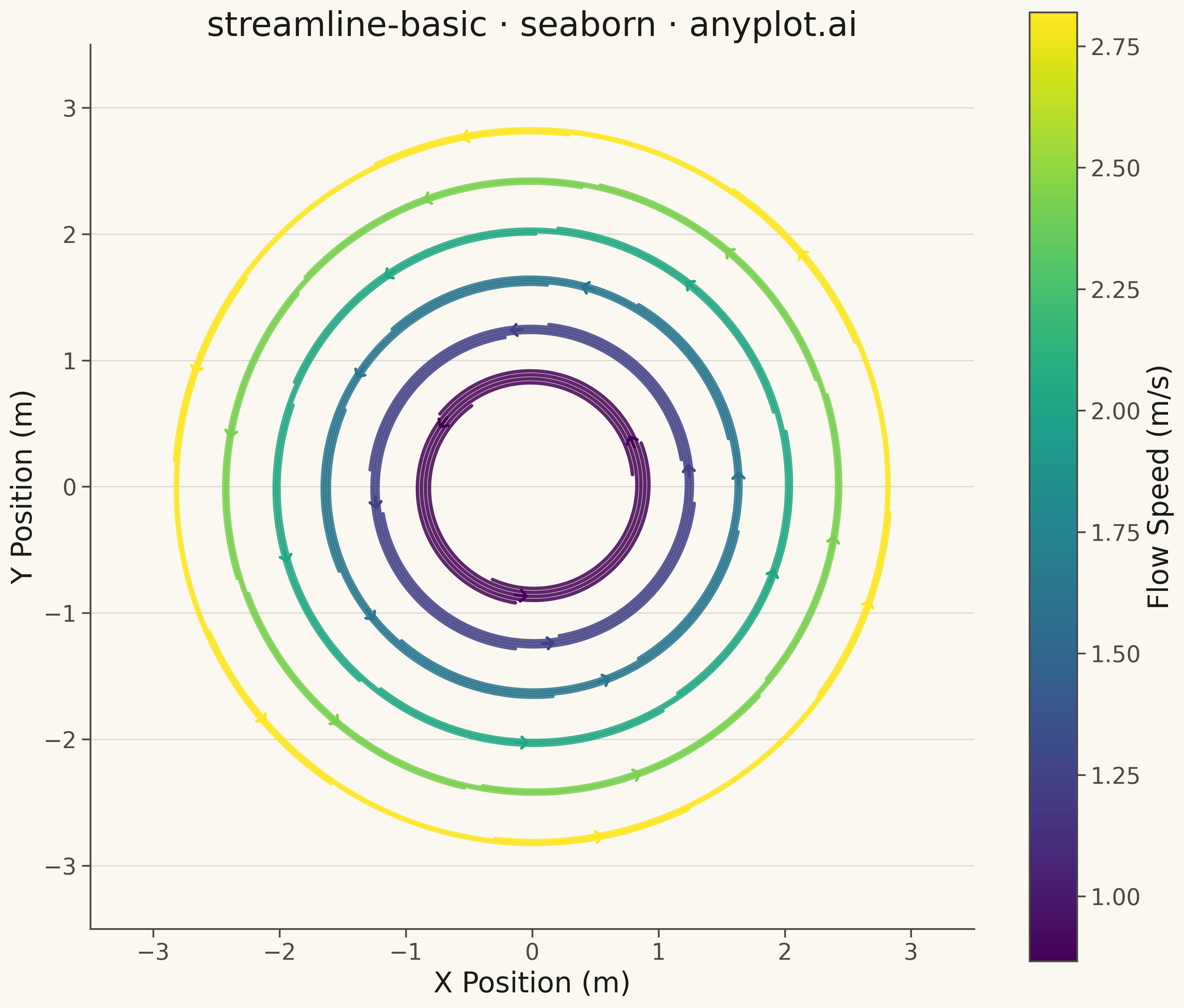
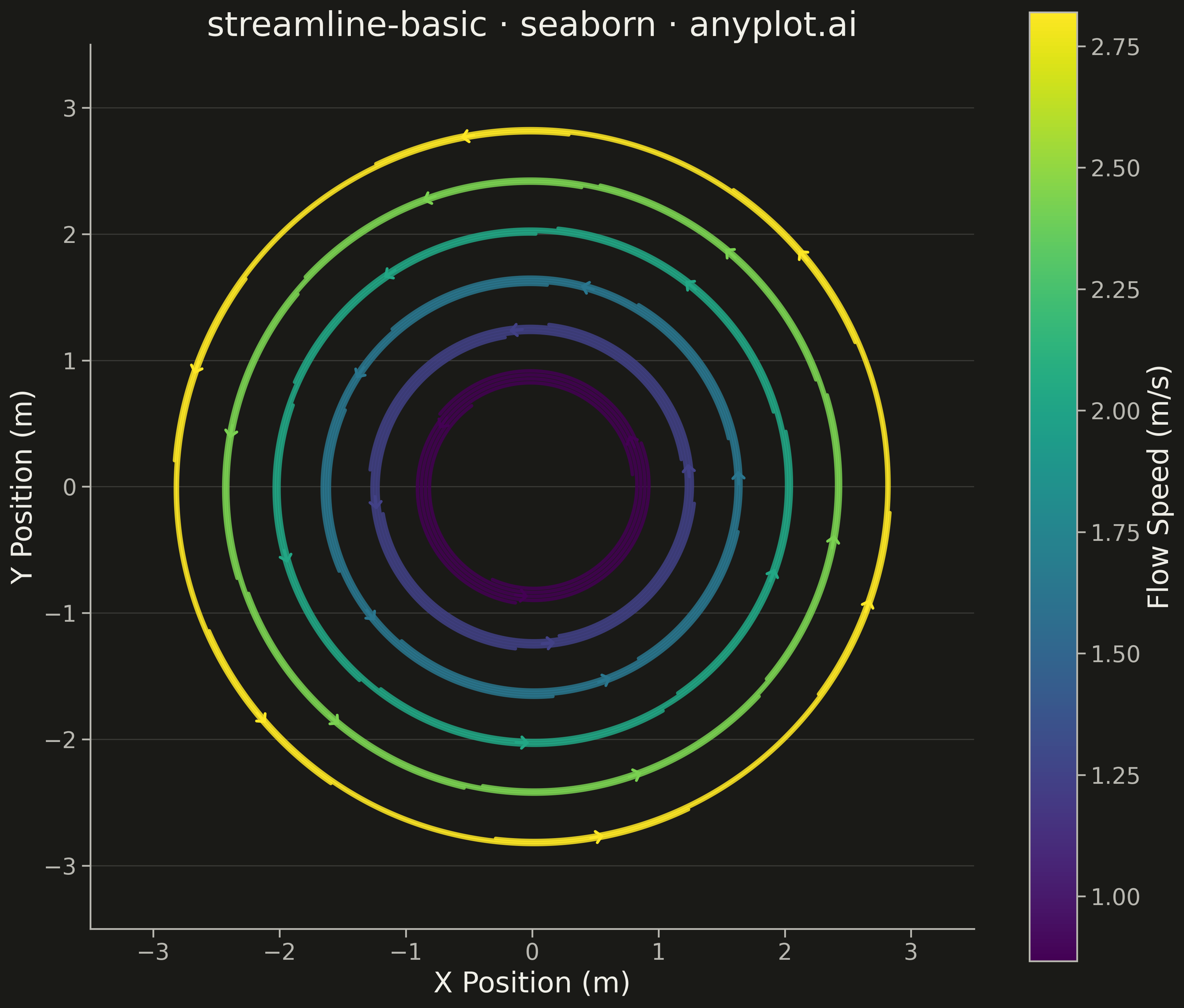
A streamline plot visualizes vector fields using smooth curves that are tangent to the field at every point. Unlike quiver plots that show discrete arrows, streamlines trace continuous paths through the field, revealing flow patterns, circulation, and field topology. This visualization is ideal for understanding fluid dynamics, electromagnetic fields, or gradient fields where the continuous nature of the flow is important.
""" anyplot.ai
streamline-basic: Basic Streamline Plot
Library: seaborn 0.13.2 | Python 3.13.13
Quality: 86/100 | Updated: 2026-05-14
"""

import os

import matplotlib.pyplot as plt
import numpy as np
import pandas as pd
import seaborn as sns
from matplotlib.patches import FancyArrowPatch


# Theme tokens
THEME = os.getenv("ANYPLOT_THEME", "light")
PAGE_BG = "#FAF8F1" if THEME == "light" else "#1A1A17"
ELEVATED_BG = "#FFFDF6" if THEME == "light" else "#242420"
INK = "#1A1A17" if THEME == "light" else "#F0EFE8"
INK_SOFT = "#4A4A44" if THEME == "light" else "#B8B7B0"

# Set seed for reproducibility
np.random.seed(42)

# Vortex flow field: u = -y, v = x (creates circular streamlines)
streamlines_data = []
arrow_data = []
streamline_id = 0

# Starting points at different radii
radii = [0.8, 1.2, 1.6, 2.0, 2.4, 2.8]
n_per_radius_map = {0.8: 3, 1.2: 4, 1.6: 5, 2.0: 5, 2.4: 6, 2.8: 6}
dt = 0.03
max_steps = 250

for r in radii:
    n_per_radius = n_per_radius_map[r]
    for i in range(n_per_radius):
        angle = 2 * np.pi * i / n_per_radius + (r * 0.15)
        x = r * np.cos(angle)
        y = r * np.sin(angle)
        streamline_points = []

        # Trace streamline using Euler integration
        for step in range(max_steps):
            if abs(x) > 3.2 or abs(y) > 3.2:
                break

            # Vector field: circular vortex
            u = -y
            v = x
            speed = np.sqrt(u**2 + v**2)

            if speed < 1e-6:
                break

            vel_mag = np.sqrt(x**2 + y**2)
            streamlines_data.append(
                {
                    "x": float(x),
                    "y": float(y),
                    "streamline_id": streamline_id,
                    "order": step,
                    "velocity": float(vel_mag),
                }
            )
            streamline_points.append((x, y, u, v, vel_mag))

            x = x + dt * u / speed
            y = y + dt * v / speed

        # Store arrow position at midpoint
        if len(streamline_points) > 20:
            mid_idx = len(streamline_points) // 2
            px, py, pu, pv, pvel = streamline_points[mid_idx]
            arrow_data.append({"x": px, "y": py, "u": pu, "v": pv, "velocity": pvel})

        streamline_id += 1

# Create DataFrames
df = pd.DataFrame(streamlines_data)
arrows_df = pd.DataFrame(arrow_data)

# Compute average velocity per streamline for color encoding
avg_velocity = df.groupby("streamline_id")["velocity"].mean().reset_index()
avg_velocity.columns = ["streamline_id", "avg_velocity"]
df = df.merge(avg_velocity, on="streamline_id")

# Configure seaborn with theme-adaptive colors
sns.set_theme(
    style="ticks",
    rc={
        "figure.facecolor": PAGE_BG,
        "axes.facecolor": PAGE_BG,
        "axes.edgecolor": INK_SOFT,
        "axes.labelcolor": INK,
        "text.color": INK,
        "xtick.color": INK_SOFT,
        "ytick.color": INK_SOFT,
        "grid.color": INK,
        "grid.alpha": 0.10,
    },
)

# Create square figure for equal aspect ratio
fig, ax = plt.subplots(figsize=(12, 12), facecolor=PAGE_BG)
ax.set_facecolor(PAGE_BG)

# Use viridis colormap for continuous velocity data
palette = sns.color_palette("viridis", as_cmap=True)
norm = plt.Normalize(df["avg_velocity"].min(), df["avg_velocity"].max())

# Plot streamlines with continuous color encoding
sns.lineplot(
    data=df,
    x="x",
    y="y",
    hue="avg_velocity",
    units="streamline_id",
    estimator=None,
    sort=False,
    linewidth=2.5,
    alpha=0.85,
    palette="viridis",
    legend=False,
    ax=ax,
)

# Add arrowheads to show flow direction
cmap = plt.cm.viridis
for _, arrow in arrows_df.iterrows():
    px, py = arrow["x"], arrow["y"]
    pu, pv = arrow["u"], arrow["v"]
    speed = np.sqrt(pu**2 + pv**2)
    dx = 0.15 * pu / speed
    dy = 0.15 * pv / speed
    color = cmap(norm(arrow["velocity"]))
    arrow_patch = FancyArrowPatch(
        (px - dx / 2, py - dy / 2),
        (px + dx / 2, py + dy / 2),
        arrowstyle="->,head_width=4,head_length=4",
        color=color,
        linewidth=2,
        mutation_scale=1,
        zorder=10,
    )
    ax.add_patch(arrow_patch)

# Add colorbar
sm = plt.cm.ScalarMappable(cmap="viridis", norm=norm)
sm.set_array([])
cbar = fig.colorbar(sm, ax=ax, shrink=0.8, aspect=20)
cbar.set_label("Flow Speed (m/s)", fontsize=20, color=INK)
cbar.ax.tick_params(labelsize=16, colors=INK_SOFT)

# Style axes
ax.set_xlabel("X Position (m)", fontsize=20, color=INK)
ax.set_ylabel("Y Position (m)", fontsize=20, color=INK)
ax.set_title("streamline-basic · seaborn · anyplot.ai", fontsize=24, fontweight="medium", color=INK)
ax.tick_params(axis="both", labelsize=16, colors=INK_SOFT)
ax.set_aspect("equal")
ax.set_xlim(-3.5, 3.5)
ax.set_ylim(-3.5, 3.5)

# Remove spines
ax.spines["top"].set_visible(False)
ax.spines["right"].set_visible(False)
ax.spines["left"].set_color(INK_SOFT)
ax.spines["bottom"].set_color(INK_SOFT)

# Subtle grid
ax.yaxis.grid(True, alpha=0.15, linewidth=0.8, color=INK)

plt.tight_layout()
plt.savefig(f"plot-{THEME}.png", dpi=300, bbox_inches="tight", facecolor=PAGE_BG)
Runnable source as JSON, for any HTTP client: https://api.anyplot.ai/specs/streamline-basic/seaborn/code. Any spec id and library id listed in llms-full.txt fit the same URL shape; every URL below is complete and callable.
{
  "spec_id": "streamline-basic",
  "language": "python",
  "library": "seaborn",
  "page": "https://anyplot.ai/streamline-basic/python/seaborn",
  "hub": "https://anyplot.ai/streamline-basic",
  "code_json": "https://api.anyplot.ai/specs/streamline-basic/seaborn/code",
  "spec_json": "https://api.anyplot.ai/specs/streamline-basic",
  "render_light_png": "https://storage.googleapis.com/anyplot-images/plots/streamline-basic/python/seaborn/plot-light.png",
  "render_dark_png": "https://storage.googleapis.com/anyplot-images/plots/streamline-basic/python/seaborn/plot-dark.png",
  "quality_score": 86.0,
  "license": "MIT",
  "guide": "https://anyplot.ai/llms.txt"
}
Part of Basic Streamline Plot on anyplot.ai.