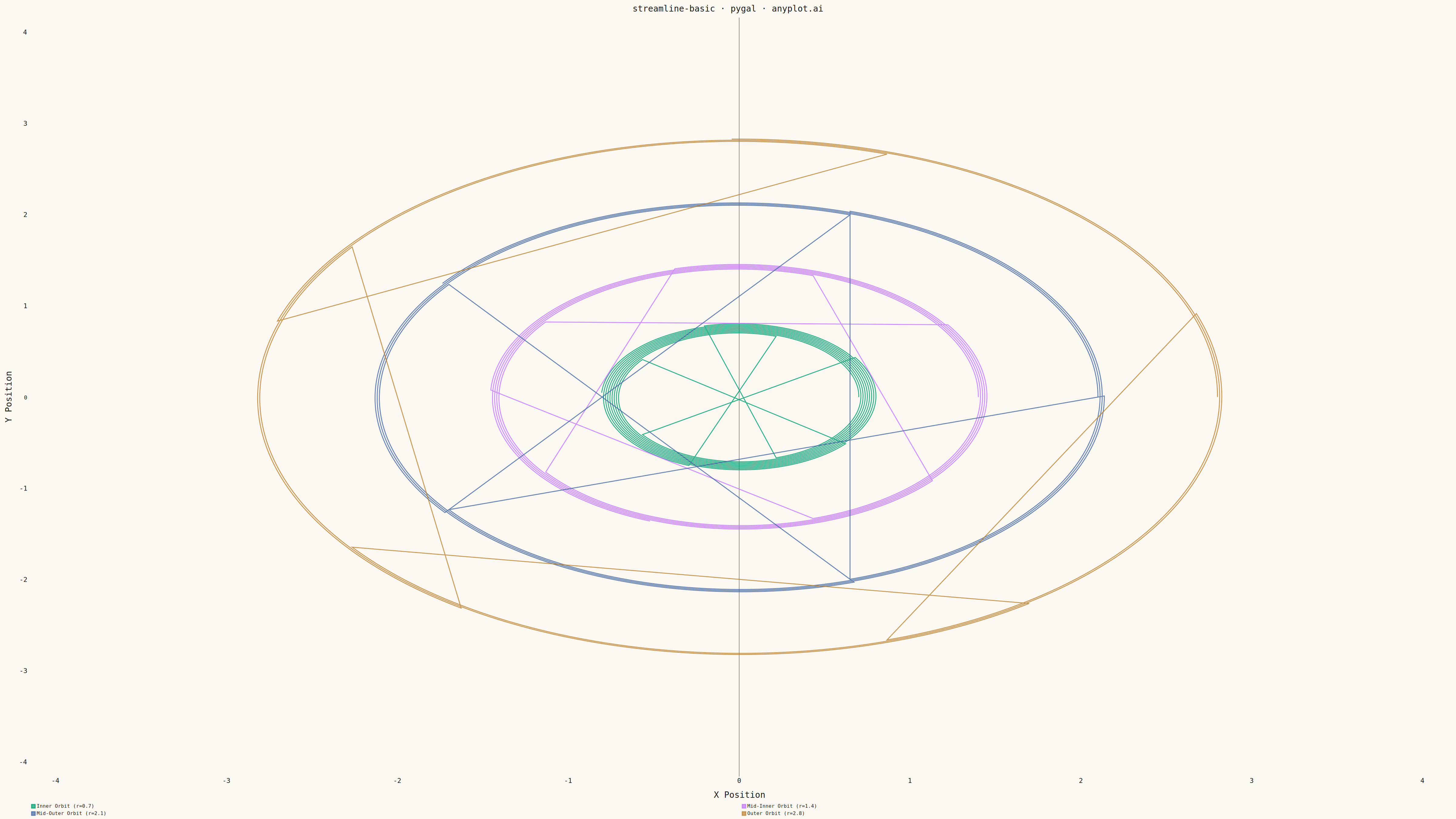
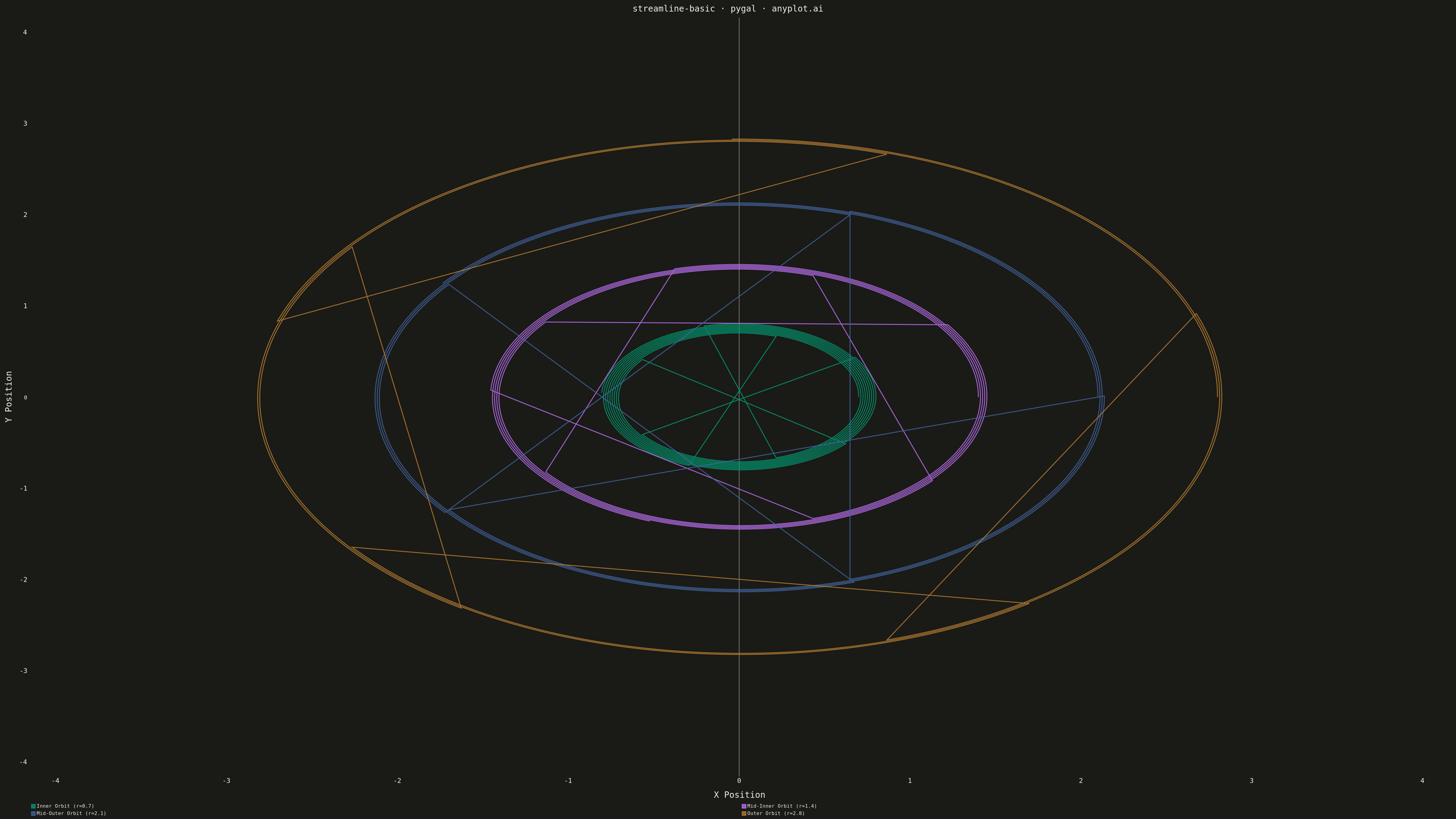
A streamline plot visualizes vector fields using smooth curves that are tangent to the field at every point. Unlike quiver plots that show discrete arrows, streamlines trace continuous paths through the field, revealing flow patterns, circulation, and field topology. This visualization is ideal for understanding fluid dynamics, electromagnetic fields, or gradient fields where the continuous nature of the flow is important.
""" anyplot.ai
streamline-basic: Basic Streamline Plot
Library: pygal 3.1.0 | Python 3.13.13
Quality: 87/100 | Updated: 2026-05-14
"""

import os
import sys

import numpy as np


# Prevent this script's directory from shadowing the pygal package
script_dir = os.path.dirname(os.path.abspath(__file__))
sys.path = [p for p in sys.path if not (p == script_dir or p == "")]

import pygal
from pygal.style import Style


# Theme tokens
THEME = os.getenv("ANYPLOT_THEME", "light")
PAGE_BG = "#FAF8F1" if THEME == "light" else "#1A1A17"
ELEVATED_BG = "#FFFDF6" if THEME == "light" else "#242420"
INK = "#1A1A17" if THEME == "light" else "#F0EFE8"
INK_SOFT = "#4A4A44" if THEME == "light" else "#B8B7B0"
INK_MUTED = "#6B6A63" if THEME == "light" else "#A8A79F"

# Okabe-Ito palette
IMPRINT = (
    "#009E73",  # Brand green - position 1
    "#C475FD",  # Vermillion - position 2
    "#4467A3",  # Blue - position 3
    "#BD8233",  # Reddish purple - position 4
)

# Data - Multiple streamline patterns to showcase varied flow
# Vortex pattern: u = -y, v = x (counterclockwise circulation)
# We'll create streamlines at different starting points

streamlines = []

# Vortex streamlines from 4 orbital radii
radii = [0.7, 1.4, 2.1, 2.8]
points_per_radius = 5

for radius_idx, radius in enumerate(radii):
    for angle_idx in range(points_per_radius):
        angle = 2 * np.pi * angle_idx / points_per_radius
        x0 = radius * np.cos(angle)
        y0 = radius * np.sin(angle)

        # Trace streamline from this starting point
        points = [(x0, y0)]
        x, y = x0, y0
        dt = 0.02
        max_steps = 400
        bounds = 3.5

        for _ in range(max_steps):
            # Velocity field: vortex with radial decay
            r = np.sqrt(x**2 + y**2)
            factor = 1.0 / (1.0 + 0.1 * r)
            u = -y * factor
            v = x * factor
            speed = np.sqrt(u**2 + v**2)

            if speed < 0.001:
                break

            # Normalize and step
            x_new = x + dt * u / speed
            y_new = y + dt * v / speed

            # Check bounds
            if abs(x_new) > bounds or abs(y_new) > bounds:
                break

            x, y = x_new, y_new
            points.append((x, y))

        if len(points) > 10:
            streamlines.append((points, radius_idx))

# Group streamlines by orbital distance
binned_streamlines = {i: [] for i in range(4)}
bin_labels = ["Inner Orbit (r=0.7)", "Mid-Inner Orbit (r=1.4)", "Mid-Outer Orbit (r=2.1)", "Outer Orbit (r=2.8)"]

for points, radius_idx in streamlines:
    binned_streamlines[radius_idx].append(points)

# Create custom style with theme-adaptive colors and proper sizing
custom_style = Style(
    background=PAGE_BG,
    plot_background=PAGE_BG,
    foreground=INK,
    foreground_strong=INK,
    foreground_subtle=INK_MUTED,
    colors=IMPRINT,
    title_font_size=28,
    label_font_size=22,
    major_label_font_size=18,
    legend_font_size=16,
    value_font_size=14,
    stroke_width=3,
)

# Create chart
chart = pygal.XY(
    style=custom_style,
    width=4800,
    height=2700,
    stroke=True,
    stroke_style={"width": 3},
    show_dots=False,
    show_legend=True,
    legend_at_bottom=True,
    legend_at_bottom_columns=2,
    title="streamline-basic · pygal · anyplot.ai",
    x_title="X Position",
    y_title="Y Position",
    show_x_guides=False,
    show_y_guides=False,
    range=(-4, 4),
    xrange=(-4, 4),
)

# Add each orbital group as a series with Okabe-Ito colors
for bin_idx in range(4):
    series_data = []
    for streamline_points in binned_streamlines[bin_idx]:
        # Add streamline points
        for point in streamline_points:
            series_data.append(point)
        # Add None to separate streamlines
        series_data.append(None)

    if series_data:
        chart.add(bin_labels[bin_idx], series_data)

# Save outputs - theme-suffixed filenames
chart.render_to_png(f"plot-{THEME}.png")
with open(f"plot-{THEME}.html", "wb") as f:
    f.write(chart.render())
Runnable source as JSON, for any HTTP client: https://api.anyplot.ai/specs/streamline-basic/pygal/code. Any spec id and library id listed in llms-full.txt fit the same URL shape; every URL below is complete and callable.
{
  "spec_id": "streamline-basic",
  "language": "python",
  "library": "pygal",
  "page": "https://anyplot.ai/streamline-basic/python/pygal",
  "hub": "https://anyplot.ai/streamline-basic",
  "code_json": "https://api.anyplot.ai/specs/streamline-basic/pygal/code",
  "spec_json": "https://api.anyplot.ai/specs/streamline-basic",
  "render_light_png": "https://storage.googleapis.com/anyplot-images/plots/streamline-basic/python/pygal/plot-light.png",
  "render_dark_png": "https://storage.googleapis.com/anyplot-images/plots/streamline-basic/python/pygal/plot-dark.png",
  "interactive_light_html": "https://storage.googleapis.com/anyplot-images/plots/streamline-basic/python/pygal/plot-light.html",
  "interactive_dark_html": "https://storage.googleapis.com/anyplot-images/plots/streamline-basic/python/pygal/plot-dark.html",
  "quality_score": 87.0,
  "license": "MIT",
  "guide": "https://anyplot.ai/llms.txt"
}
Part of Basic Streamline Plot on anyplot.ai.