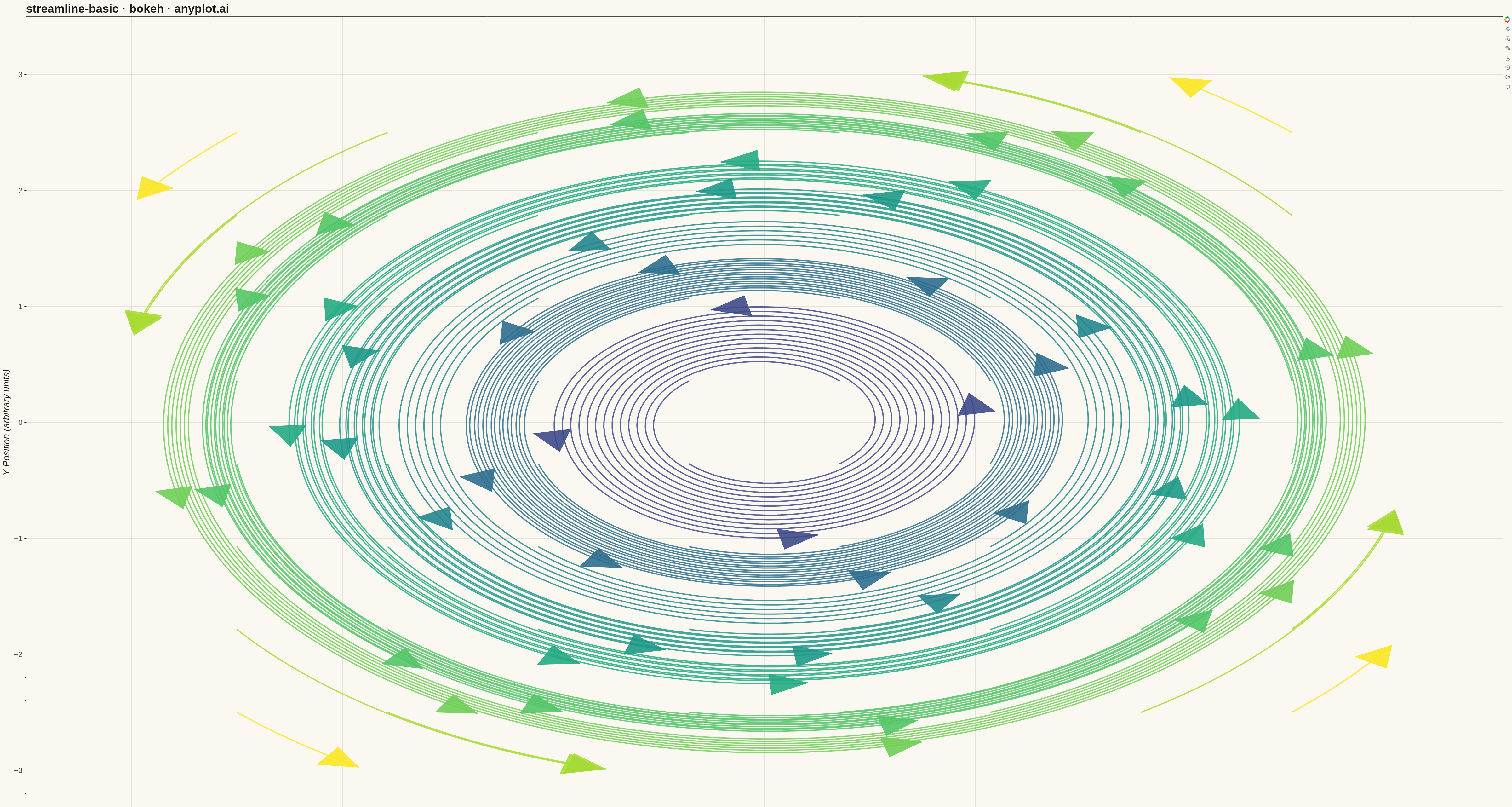
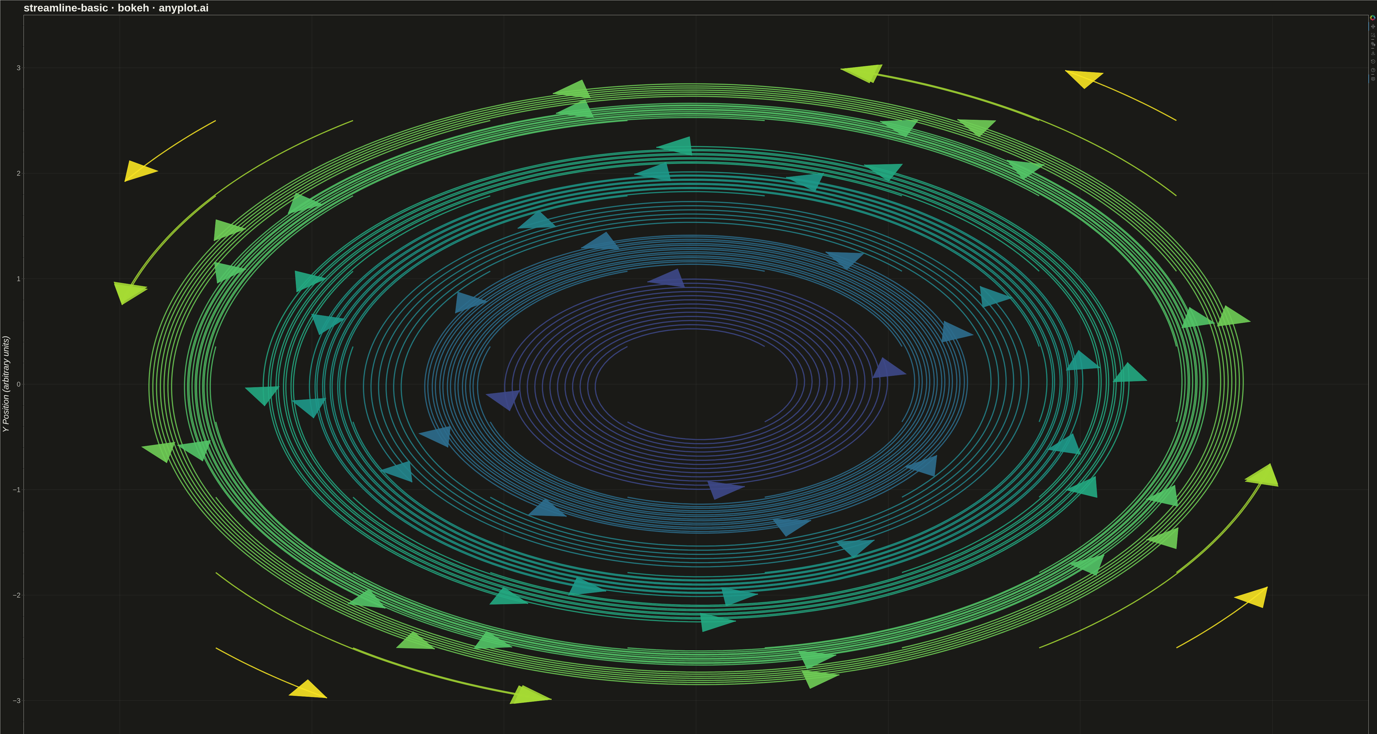
A streamline plot visualizes vector fields using smooth curves that are tangent to the field at every point. Unlike quiver plots that show discrete arrows, streamlines trace continuous paths through the field, revealing flow patterns, circulation, and field topology. This visualization is ideal for understanding fluid dynamics, electromagnetic fields, or gradient fields where the continuous nature of the flow is important.
""" anyplot.ai
streamline-basic: Basic Streamline Plot
Library: bokeh 3.9.0 | Python 3.13.13
Quality: 95/100 | Updated: 2026-05-14
"""

import os
import time
from importlib import import_module
from pathlib import Path

import numpy as np
from scipy.interpolate import RegularGridInterpolator
from selenium import webdriver
from selenium.webdriver.chrome.options import Options


bokeh_io = import_module("bokeh.io")
bokeh_models = import_module("bokeh.models")
bokeh_palettes = import_module("bokeh.palettes")
bokeh_plotting = import_module("bokeh.plotting")

output_file = bokeh_io.output_file
save = bokeh_io.save
HoverTool = bokeh_models.HoverTool
Viridis256 = bokeh_palettes.Viridis256
figure = bokeh_plotting.figure

# Theme tokens
THEME = os.getenv("ANYPLOT_THEME", "light")
PAGE_BG = "#FAF8F1" if THEME == "light" else "#1A1A17"
ELEVATED_BG = "#FFFDF6" if THEME == "light" else "#242420"
INK = "#1A1A17" if THEME == "light" else "#F0EFE8"
INK_SOFT = "#4A4A44" if THEME == "light" else "#B8B7B0"

# Seed for reproducibility
np.random.seed(42)

# Grid setup
x = np.linspace(-3, 3, 40)
y = np.linspace(-3, 3, 40)
X, Y = np.meshgrid(x, y)

# Vortex flow field: u = -y, v = x (creates circular streamlines)
U = -Y
V = X

# Compute velocity magnitude for coloring
magnitude = np.sqrt(U**2 + V**2)

# Create interpolators for the vector field
u_interp = RegularGridInterpolator((y, x), U, bounds_error=False, fill_value=None)
v_interp = RegularGridInterpolator((y, x), V, bounds_error=False, fill_value=None)
mag_interp = RegularGridInterpolator((y, x), magnitude, bounds_error=False, fill_value=None)

# Seed points for streamlines in a grid pattern
seed_x = np.linspace(-2.5, 2.5, 8)
seed_y = np.linspace(-2.5, 2.5, 8)

# Storage for streamline data
streamlines_data = []

# Compute streamlines from seed points
for sx in seed_x:
    for sy in seed_y:
        # Trace streamline using Euler integration
        xs, ys, mags = [sx], [sy], []
        px, py = sx, sy
        dt, max_steps = 0.05, 300

        # Get initial magnitude
        m = mag_interp([[py, px]])[0]
        if m is None or np.isnan(m):
            continue
        mags.append(m)

        for _ in range(max_steps):
            u_val = u_interp([[py, px]])[0]
            v_val = v_interp([[py, px]])[0]

            if u_val is None or v_val is None or np.isnan(u_val) or np.isnan(v_val):
                break

            speed = np.sqrt(u_val**2 + v_val**2)
            if speed < 1e-6:
                break

            # Normalize and step
            px += u_val / speed * dt
            py += v_val / speed * dt

            # Check bounds
            if px < x.min() or px > x.max() or py < y.min() or py > y.max():
                break

            xs.append(px)
            ys.append(py)
            m = mag_interp([[py, px]])[0]
            if m is None or np.isnan(m):
                break
            mags.append(m)

        # Store if streamline is long enough
        if len(xs) >= 5:
            avg_mag = np.mean(mags)
            streamlines_data.append(
                {"xs": np.array(xs), "ys": np.array(ys), "mags": np.array(mags), "avg_mag": avg_mag}
            )

# Create figure
p = figure(
    width=4800,
    height=2700,
    title="streamline-basic · bokeh · anyplot.ai",
    x_axis_label="X Position (arbitrary units)",
    y_axis_label="Y Position (arbitrary units)",
    x_range=(-3.5, 3.5),
    y_range=(-3.5, 3.5),
)

# Style title and axes for large canvas
p.title.text_font_size = "28pt"
p.title.text_color = INK
p.xaxis.axis_label_text_font_size = "22pt"
p.yaxis.axis_label_text_font_size = "22pt"
p.xaxis.axis_label_text_color = INK
p.yaxis.axis_label_text_color = INK
p.xaxis.major_label_text_font_size = "18pt"
p.yaxis.major_label_text_font_size = "18pt"
p.xaxis.major_label_text_color = INK_SOFT
p.yaxis.major_label_text_color = INK_SOFT

# Grid styling
p.xgrid.grid_line_color = INK
p.ygrid.grid_line_color = INK
p.xgrid.grid_line_alpha = 0.10
p.ygrid.grid_line_alpha = 0.10

# Spine colors
p.outline_line_color = INK_SOFT
p.xaxis.axis_line_color = INK_SOFT
p.yaxis.axis_line_color = INK_SOFT
p.xaxis.major_tick_line_color = INK_SOFT
p.yaxis.major_tick_line_color = INK_SOFT

# Background
p.background_fill_color = PAGE_BG
p.border_fill_color = PAGE_BG

# Normalize magnitude for color mapping (0-1 scale for Viridis256)
max_mag = max(s["avg_mag"] for s in streamlines_data)
if max_mag > 0:
    norm_mags = [s["avg_mag"] / max_mag for s in streamlines_data]
else:
    norm_mags = [0.5 for _ in streamlines_data]

# Draw streamlines with direction arrows
for sl_data, norm_mag in zip(streamlines_data, norm_mags, strict=False):
    xs = sl_data["xs"]
    ys = sl_data["ys"]

    # Map normalized magnitude to Viridis256 color
    color_idx = min(int(norm_mag * 255), 255)
    color = Viridis256[color_idx]

    # Draw streamline
    p.line(xs, ys, line_width=4, line_color=color, line_alpha=0.85)

    # Add arrowhead at the end to show flow direction
    if len(xs) >= 2:
        dx = xs[-1] - xs[-2]
        dy = ys[-1] - ys[-2]
        length = np.sqrt(dx**2 + dy**2)
        if length > 0:
            dx /= length
            dy /= length
            arrow_size = 0.18
            tip_x, tip_y = xs[-1], ys[-1]
            wing1_x = tip_x - arrow_size * (dx + 0.5 * dy)
            wing1_y = tip_y - arrow_size * (dy - 0.5 * dx)
            wing2_x = tip_x - arrow_size * (dx - 0.5 * dy)
            wing2_y = tip_y - arrow_size * (dy + 0.5 * dx)
            p.patch(
                [tip_x, wing1_x, wing2_x], [tip_y, wing1_y, wing2_y], fill_color=color, line_color=color, fill_alpha=0.9
            )

# Add hover tool for interactivity
hover = HoverTool(tooltips=[("Position", "($x, $y)")])
p.add_tools(hover)

# Save HTML (required artifact)
output_file(f"plot-{THEME}.html")
save(p)

# Screenshot with headless Chrome for PNG
W, H = 4800, 2700
opts = Options()
for arg in (
    "--headless=new",
    "--no-sandbox",
    "--disable-dev-shm-usage",
    "--disable-gpu",
    f"--window-size={W},{H}",
    "--hide-scrollbars",
):
    opts.add_argument(arg)
driver = webdriver.Chrome(options=opts)
driver.set_window_size(W, H)
driver.get(f"file://{Path(f'plot-{THEME}.html').resolve()}")
time.sleep(3)
driver.save_screenshot(f"plot-{THEME}.png")
driver.quit()
Runnable source as JSON, for any HTTP client: https://api.anyplot.ai/specs/streamline-basic/bokeh/code. Any spec id and library id listed in llms-full.txt fit the same URL shape; every URL below is complete and callable.
{
  "spec_id": "streamline-basic",
  "language": "python",
  "library": "bokeh",
  "page": "https://anyplot.ai/streamline-basic/python/bokeh",
  "hub": "https://anyplot.ai/streamline-basic",
  "code_json": "https://api.anyplot.ai/specs/streamline-basic/bokeh/code",
  "spec_json": "https://api.anyplot.ai/specs/streamline-basic",
  "render_light_png": "https://storage.googleapis.com/anyplot-images/plots/streamline-basic/python/bokeh/plot-light.png",
  "render_dark_png": "https://storage.googleapis.com/anyplot-images/plots/streamline-basic/python/bokeh/plot-dark.png",
  "interactive_light_html": "https://storage.googleapis.com/anyplot-images/plots/streamline-basic/python/bokeh/plot-light.html",
  "interactive_dark_html": "https://storage.googleapis.com/anyplot-images/plots/streamline-basic/python/bokeh/plot-dark.html",
  "quality_score": 95.0,
  "license": "MIT",
  "guide": "https://anyplot.ai/llms.txt"
}
Part of Basic Streamline Plot on anyplot.ai.